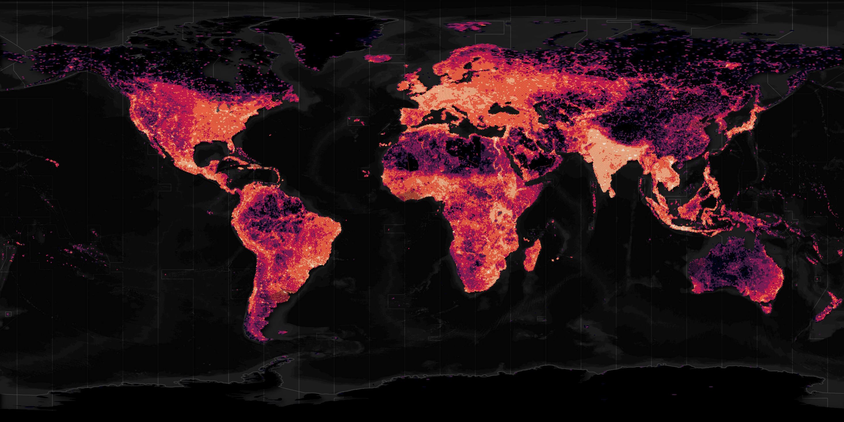
On Monday last week, a paper was published announcing the OpenBuildingMap (OBM) dataset. With varying degrees of coverage, it contains building footprints, heights, 8 categories of usage and floorspace for 2.7B buildings across the globe. Below is a heatmap of its building footprints.
Existing data from OpenStreetMap (OSM), Google's Open Buildings, Microsoft Global ML Building Footprints and the Global Human Settlement Characteristics Layer were used to build this dataset. OBM's paper states the authors didn't use the CLSM dataset for East Asia due to uncertain licensing regarding the imagery that dataset was built from.
Efforts were made to clean up the data including removing buildings located over water bodies and excluding height information from any building claiming to be taller that the world's tallest tower, the Burj Khalifa in Dubai.
OBM is broken up into 1,270 BZip2-compressed GeoPackage (GPKG) files. I downloaded these and converted them into ZStandard-compressed, spatial-sorted Parquet files. These are now being hosted on AWS S3 thanks to the kind generosity of Source Cooperative and Taylor Geospatial Engine.
GPKG files are great if you're going to edit the data but for analysis, surgical downloading and archiving, it's really hard to beat Parquet. Parquet stores data as columns and has statistics for groups of rows in each column, often every 10-100K rows. This means some analytical queries only need a few MBs of bandwidth to analyse GBs or TBs of data stored remotely on AWS S3 or HTTPS-based CDNs like Cloudflare's.
GPKG files are based on SQLite and are row-oriented so compressing them rarely reduces the file size by more than a 5:1 ratio. With columnar formats like Parquet, 15:1 reductions are the norm. Decompressing the BZip2 files in this post maxed out around 10MB/s on my system. ZStandard runs circles around this.
In this post, I'll walk through converting this dataset into Parquet and examining some of its features.
My Workstation
I'm using a 5.7 GHz AMD Ryzen 9 9950X CPU. It has 16 cores and 32 threads and 1.2 MB of L1, 16 MB of L2 and 64 MB of L3 cache. It has a liquid cooler attached and is housed in a spacious, full-sized Cooler Master HAF 700 computer case.
The system has 96 GB of DDR5 RAM clocked at 4,800 MT/s and a 5th-generation, Crucial T700 4 TB NVMe M.2 SSD which can read at speeds up to 12,400 MB/s. There is a heatsink on the SSD to help keep its temperature down. This is my system's C drive.
The system is powered by a 1,200-watt, fully modular Corsair Power Supply and is sat on an ASRock X870E Nova 90 Motherboard.
I'm running Ubuntu 24 LTS via Microsoft's Ubuntu for Windows on Windows 11 Pro. In case you're wondering why I don't run a Linux-based desktop as my primary work environment, I'm still using an Nvidia GTX 1080 GPU which has better driver support on Windows and ArcGIS Pro only supports Windows natively.
Installing Prerequisites
I'll use GDAL 3.9.3 and a few other tools to help analyse the data in this post.
$ sudo add-apt-repository ppa:ubuntugis/ubuntugis-unstable
$ sudo apt update
$ sudo apt install \
    gdal-bin \
    jq
I'll use DuckDB, along with its H3, JSON, Lindel, Parquet and Spatial extensions in this post.
$ cd ~
$ wget -c https://github.com/duckdb/duckdb/releases/download/v1.4.1/duckdb_cli-linux-amd64.zip
$ unzip -j duckdb_cli-linux-amd64.zip
$ chmod +x duckdb
$ ~/duckdb
INSTALL h3 FROM community;
INSTALL lindel FROM community;
INSTALL json;
INSTALL parquet;
INSTALL spatial;
I'll set up DuckDB to load every installed extension each time it launches.
$ vi ~/.duckdbrc
.timer on
.width 180
LOAD h3;
LOAD lindel;
LOAD json;
LOAD parquet;
LOAD spatial;
The maps in this post were rendered with QGIS version 3.44. QGIS is a desktop application that runs on Windows, macOS and Linux. The application has grown in popularity in recent years and has ~15M application launches from users all around the world each month.
The dark heatmaps in this post are mostly made up of vector data from Natural Earth and Overture.
Downloading the Buildings
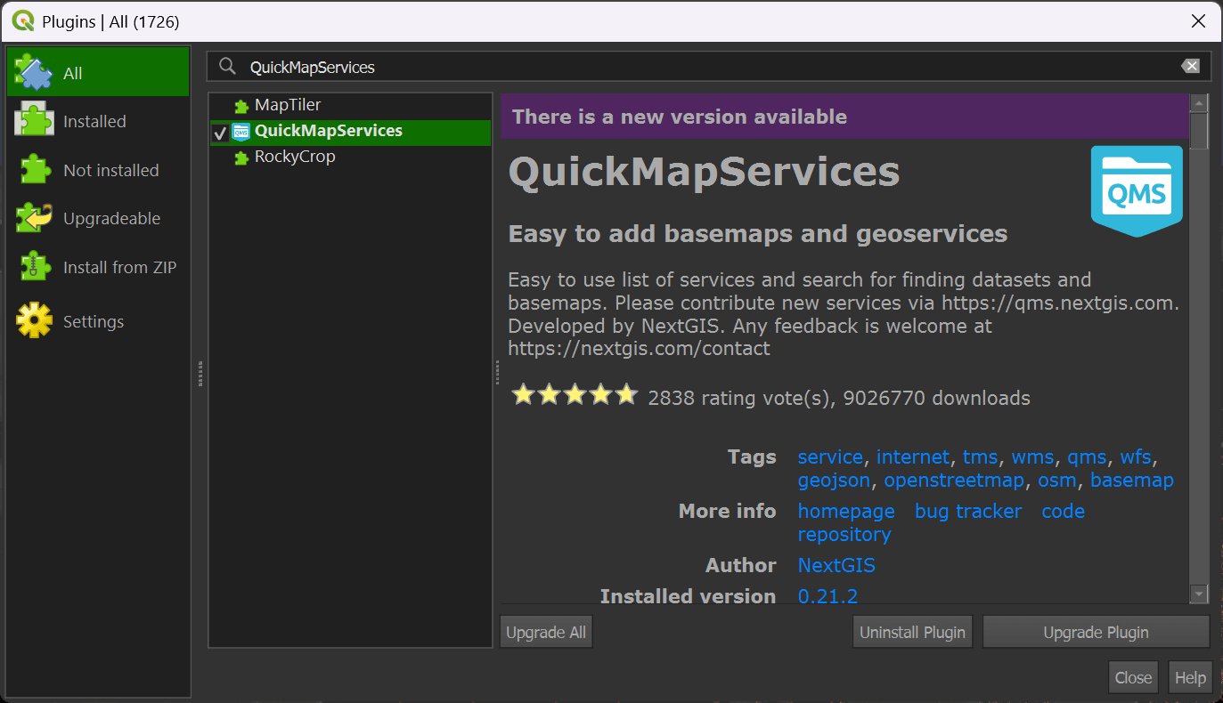
In QGIS, click the "Plugins" Menu and then the "Manage and Install Plugins" item. Click the "All" filter in the top left of the dialog and then search for "QuickMapServices". Click to install or upgrade the plugin in the bottom right of the dialog.
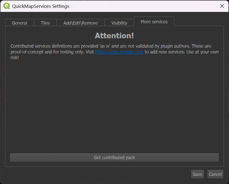
Click the "Web" Menu, then "QuickMapServices" and then the "Settings" item. Click the "More Services" tab at the top of the dialog. Click the "Get contributed pack" button.
In the "Web" menu under "QuickMapServices" you should now see the list of several basemap providers.
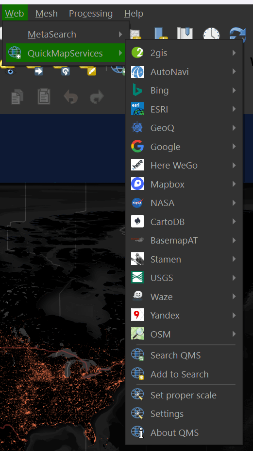
Select "OSM" and then "OSM Standard" to add a world map to your scene.
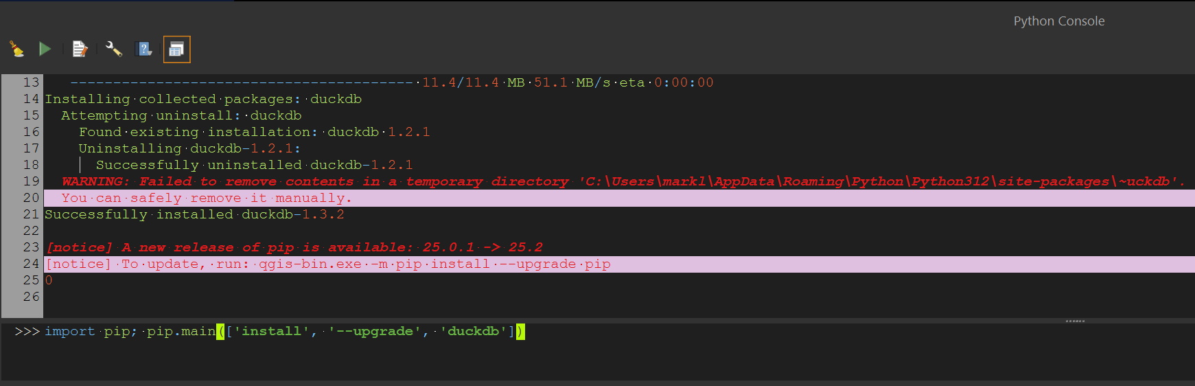
Under the "Plugins" menu, select "Python Console". Paste in the following line of Python. It'll ensure you've got the latest version of DuckDB installed in QGIS' Python Environment.
import pip; pip.main(['install', '--upgrade', 'duckdb'])
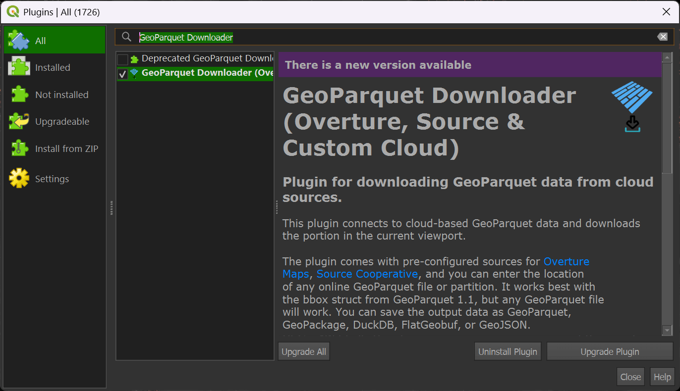
In QGIS, click the "Plugins" Menu and then the "Manage and Install Plugins" item. Click the "All" filter in the top left of the dialog and then search for "GeoParquet Downloader". Click to install or upgrade the plugin in the bottom right of the dialog.
Zoom into a city of interest somewhere in the world. It's important to make sure you're not looking at an area larger than a major city as the viewport will set the boundaries for how much data will be downloaded.
If you can see the whole earth, GeoParquet Downloader will end up downloading 194 GB of data. Downloading only a city's worth of data will likely only need a few MB of data.
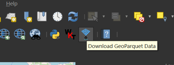
In your toolbar, click on the GeoParquet Downloader icon. It's the one with blue, rotated rectangles.
Click the "Custom URL" option and paste the following URL in.
s3://us-west-2.opendata.source.coop/tge-labs/openbuildingmap/*.parquet
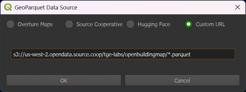
Hit "OK". You'll be prompted to save a Parquet file onto your computer. Once you've done so, the building data for your map's footprint should appear shortly afterword.
Once the buildings have loaded, select the layer styling for the downloaded buildings layer. The combo box at the top of the styling panel should be switched from "Single Symbol" to "2.5D".
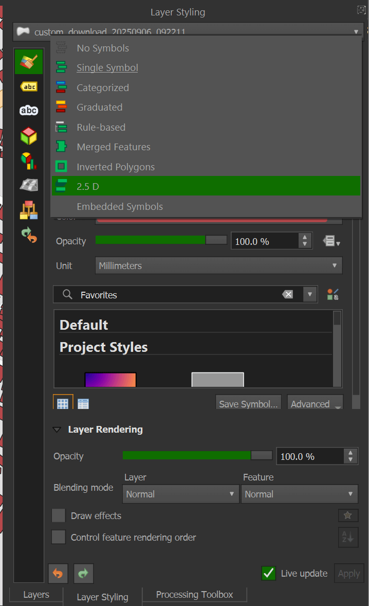
I've set the roof colour to #b13327, wall colour to #4f090b, angle to 230 degrees and added a drop shadow effect to the layer.
In the "Height" field, change it to the following expression:
if(string_to_array(height, ':')[0] = 'H', string_to_array(height, ':')[1], 1) / 50000
You should now see a 2.5D representation of the buildings you downloaded.
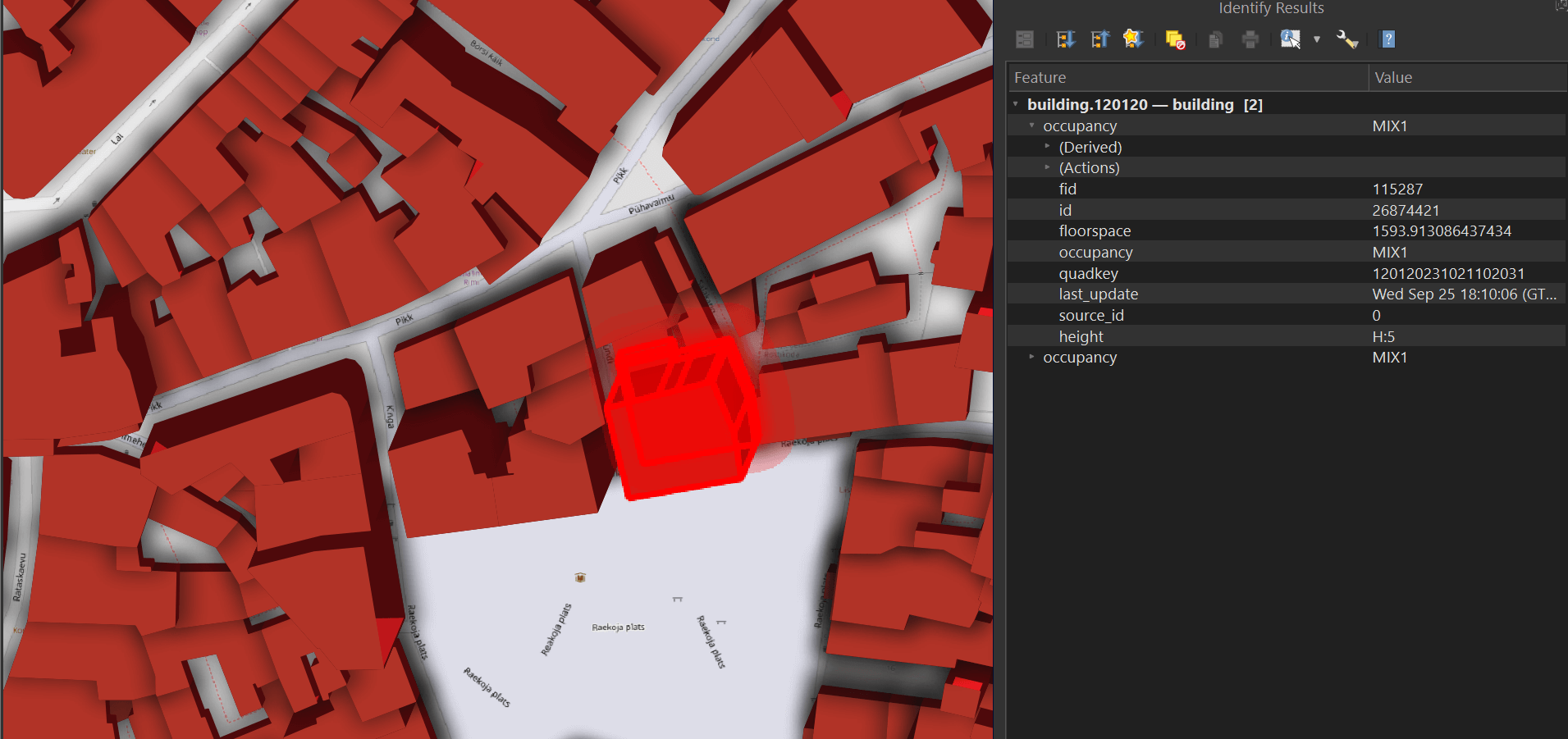
There is an "Identify Features" icon in the toolbar.
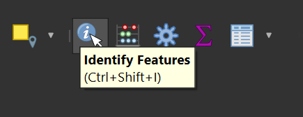
This tool lets you select any building and bring up its metadata.
The Parquet file you saved can also be read via DuckDB and even dropped into Esri's ArcGIS Pro 3.5 or newer if you have it installed on your machine.
Downloading OpenBuildingMap
Below I'll show how I turned the GPKG files into Parquet. These steps don't need to be repeated as the resulting files are now on S3.
OBM has a website where you can see the footprints of their GPKG files and download them individually. I found a GeoJSON-formatted manifest file used by the site. It contains the URLs for all of their BZ2-compressed GPKG files.
$ mkdir -p ~/obm
$ cd ~/obm

$ curl -S 'https://umap.openstreetmap.de/de/datalayer/81684/ac9788a9-c215-417d-a580-cb545acd78b9/' \
    > manifest.json
Below is an example record from this manifest.
$ echo "SELECT a.properties::JSON
        FROM (SELECT UNNEST(features) a
              FROM   READ_JSON('manifest.json'))
        LIMIT 1" \
    | ~/duckdb -json \
    | jq -S .
[
  {
    "CAST(a.properties AS \"JSON\")": {
      "URL": "https://datapub.gfz.de/download/10.5880.GFZ.LKUT.2025.002-Caweb/2025-002_Oostwegel-et-al_data/building.002202.gpkg.bz2",
      "completeness_index": 92.93,
      "fid": 1,
      "filename": "building.002202.gpkg",
      "license": "ODbL",
      "number_of_buildings": 127,
      "percentage_known_floorspace": 0.0,
      "percentage_known_height": 3.94,
      "percentage_known_occupancy": 47.24,
      "percentage_source_google": 0.0,
      "percentage_source_microsoft": 0.0,
      "percentage_source_openstreetmap": 100.0,
      "quadkey": "002202"
    }
  }
]
I'll build a list of URLs and use wget to download them with a concurrency of four.
$ echo "SELECT a.properties.URL
        FROM (SELECT UNNEST(features) a
              FROM   READ_JSON('manifest.json'))" \
    | ~/duckdb -csv \
               -noheader \
    > manifest.txt

$ cat manifest.txt \
    | xargs -P4 \
            -I% \
            wget -c "%"
GPKG to Parquet
The following converted 278 GB worth of BZip2 files containing ~722 GB worth of GPKG data into 194 GB of Parquet containing 2,693,211,269 records. Even with 24 concurrent processes running, it took the better part of a day to complete.
$ ls building.*.gpkg.bz2 \
    | xargs -P24 \
            -I% \
            bash -c "
    BASENAME=\`echo \"%\" | cut -f2 -d.\`
    PQ_FILE=\"building.\$BASENAME.parquet\"

    if [ ! -f \$PQ_FILE ]; then
        echo \"Building \$PQ_FILE.\"

        bzip2 -dk \"%\" --stdout > \"working.\$BASENAME.gpkg\"

        echo \"COPY (
                   SELECT   * EXCLUDE (geom,
                                       source_id),
                            geometry: geom,
                            bbox:     {'xmin': ST_XMIN(ST_EXTENT(geom)),
                                       'ymin': ST_YMIN(ST_EXTENT(geom)),
                                       'xmax': ST_XMAX(ST_EXTENT(geom)),
                                       'ymax': ST_YMAX(ST_EXTENT(geom))},
                            source:   CASE WHEN source_id = 0 THEN 'OSM'
                                           WHEN source_id = 1 THEN 'Google'
                                           WHEN source_id = 2 THEN 'Microsoft'
                                      END
                   FROM     ST_READ('working.\$BASENAME.gpkg')
                   ORDER BY HILBERT_ENCODE([
                                ST_Y(ST_CENTROID(geom)),
                                ST_X(ST_CENTROID(geom))]::double[2])
                ) TO '\$PQ_FILE' (
                    FORMAT            'PARQUET',
                    CODEC             'ZSTD',
                    COMPRESSION_LEVEL 22,
                    ROW_GROUP_SIZE    15000);\" \
                | ~/duckdb

        rm \"working.\$BASENAME.gpkg\"
    else
        echo \"\$PQ_FILE already exists, skipping..\"
    fi"
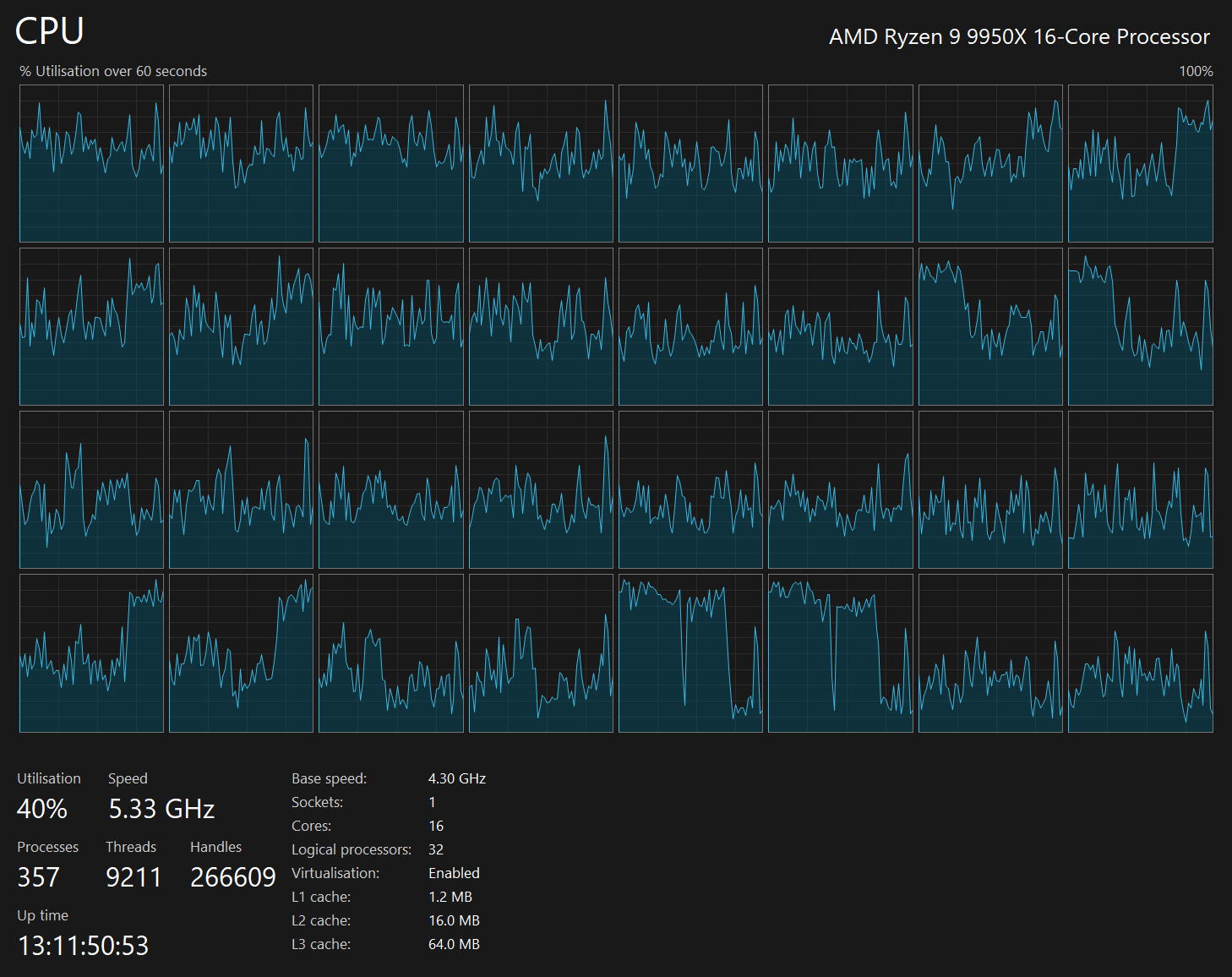
Below is what my system's CPU usage looked like while the above was running.
Data Fluency
The following is an example record from this dataset.
$ echo "SELECT * EXCLUDE(bbox),
               bbox::JSON AS bbox
        FROM   'building.*.parquet'
        WHERE  floorspace IS NOT NULL
        LIMIT  1" \
    | ~/duckdb -json \
    | jq -S .
[
  {
    "bbox": {
      "xmax": -160.03150641447675,
      "xmin": -160.03228425509127,
      "ymax": 70.63789626901166,
      "ymin": 70.63765269090544
    },
    "floorspace": "719.5123100951314",
    "geometry": "POLYGON ((-160.03228425509127 70.63772552964403, -160.03180145746848 70.63789626901166, -160.03150641447675 70.63781446163671, -160.0315654230751 70.6377735579492, -160.0318229151406 70.63767574113916, -160.0319946603366 70.63765269090544, -160.03228425509127 70.63772552964403))",
    "height": "H:2",
    "id": 500236864,
    "last_update": "2024-09-25 17:23:12.186+03",
    "occupancy": "RES3",
    "quadkey": "002213322233003100",
    "relation_id": null,
    "source": "OSM"
  }
]
Below are the field names, data types, percentages of NULLs per column, number of unique values and minimum and maximum values for each column.
$ ~/duckdb
SELECT   column_name,
         column_type,
         null_percentage,
         approx_unique,
         min,
         max
FROM     (SUMMARIZE
          FROM 'building.*.parquet')
WHERE    column_name != 'geometry'
AND      column_name != 'bbox'
ORDER BY 1;
┌─────────────┬──────────────────────────┬─────────────────┬───────────────┬────────────────────────────┬───────────────────────────┐
│ column_name │       column_type        │ null_percentage │ approx_unique │            min             │            max            │
│   varchar   │         varchar          │  decimal(9,2)   │     int64     │          varchar           │          varchar          │
├─────────────┼──────────────────────────┼─────────────────┼───────────────┼────────────────────────────┼───────────────────────────┤
│ floorspace  │ VARCHAR                  │           98.81 │      31981048 │ -4.910890285223722         │ 9999.999575164324         │
│ height      │ VARCHAR                  │           24.78 │         31689 │ H:1                        │ HHT:99.95                 │
│ id          │ BIGINT                   │            0.00 │    1985306599 │ -17787084                  │ 2304182979                │
│ last_update │ TIMESTAMP WITH TIME ZONE │            0.00 │      18555352 │ 2024-09-25 17:23:12.185+03 │ 2024-10-09 15:08:17.53+03 │
│ occupancy   │ VARCHAR                  │            0.00 │            42 │ AGR                        │ UNK                       │
│ quadkey     │ VARCHAR                  │            0.00 │     354530921 │ 002202022321313300         │ 331301200330323102        │
│ relation_id │ VARCHAR                  │           99.99 │         57371 │ -10000436.0                │ 998911012.0               │
│ source      │ VARCHAR                  │            0.00 │             3 │ Google                     │ OSM                       │
└─────────────┴──────────────────────────┴─────────────────┴───────────────┴────────────────────────────┴───────────────────────────┘
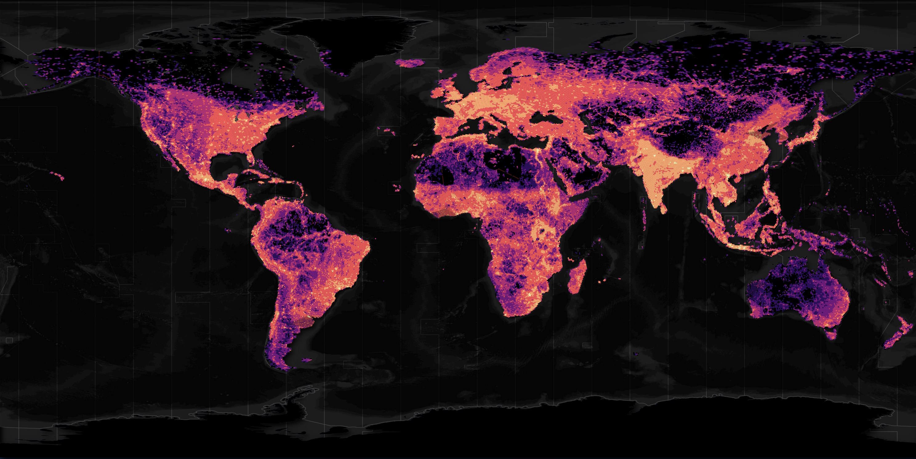
I'll generate a heatmap of the building footprints in this dataset.
$ ~/duckdb obm.duckdb
CREATE OR REPLACE TABLE h3_4_stats AS
    SELECT   H3_LATLNG_TO_CELL(
                bbox.ymin,
                bbox.xmin, 4) AS h3_4,
             COUNT(*) num_buildings
    FROM     'building.*.parquet'
    GROUP BY 1;

COPY (
    SELECT ST_ASWKB(H3_CELL_TO_BOUNDARY_WKT(h3_4)::geometry) geometry,
           num_buildings
    FROM   h3_4_stats
    WHERE  ST_XMIN(geometry::geometry) BETWEEN -179 AND 179
    AND    ST_XMAX(geometry::geometry) BETWEEN -179 AND 179
) TO 'h3_4_stats.parquet' (
        FORMAT 'PARQUET',
        CODEC  'ZSTD',
        COMPRESSION_LEVEL 22,
        ROW_GROUP_SIZE 15000);
There are very few Chinese buildings in this dataset.
Below is the TUM dataset which used satellite imagery of China to help detect as many building footprints as possible. The heatmap below shows China's South East has a building density on par with most of its neighbouring countries.
Building Uses
There are eight different building use classifications in this dataset. The uses and their acronyms are residential (RES), commercial and public (COM), mixed use (MIX), industrial (IND), agricultural (AGR), assembly (ASS), government (GOV) and education (EDU). UNK stands for unknown and accounts for ~60% of the buildings in this dataset.
After the 3-letter building use acronym there can be suffixes that provide more detail, such as RES2, which means the residential building is an apartment building. The "Building occupancy type" section of the paper goes into more detail.
Below are the building counts by use and suffix.
WITH a AS (
    SELECT   num_recs: COUNT(*),
             use:      occupancy[:3],
             use_ext:  occupancy[4:]
    FROM     'building.*.parquet'
    GROUP BY 2, 3
    ORDER BY 2, 3
)
PIVOT    a
ON       use
USING    SUM(num_recs)
GROUP BY use_ext
ORDER BY TRY_CAST(REGEXP_REPLACE(use_ext, '[A-Z]', '') AS INT);
┌─────────┬──────────┬─────────┬─────────┬─────────┬─────────┬──────────┬─────────┬───────────┬────────────┐
│ use_ext │   AGR    │   ASS   │   COM   │   EDU   │   GOV   │   IND    │   MIX   │    RES    │    UNK     │
│ varchar │  int128  │ int128  │ int128  │ int128  │ int128  │  int128  │ int128  │  int128   │   int128   │
├─────────┼──────────┼─────────┼─────────┼─────────┼─────────┼──────────┼─────────┼───────────┼────────────┤
│ 1       │   785006 │ 1982076 │ 4053587 │   93893 │  516140 │   934295 │ 4072344 │  64826183 │       NULL │
│ 2A      │     NULL │    NULL │    NULL │    NULL │    NULL │     NULL │    NULL │    120885 │       NULL │
│ 2       │   189285 │  182617 │  161023 │ 5513273 │  190597 │    15282 │    9524 │   8874805 │       NULL │
│ 3       │  1199083 │   22159 │  422796 │ 1813089 │    NULL │     NULL │    NULL │  16615755 │       NULL │
│ 4       │     NULL │  106813 │ 1774918 │    8714 │    NULL │     NULL │ 1833277 │     32207 │       NULL │
│ 5       │     NULL │    NULL │  643386 │    NULL │    NULL │     NULL │  724050 │      NULL │       NULL │
│ 6       │     NULL │    NULL │  200419 │    NULL │    NULL │     NULL │    NULL │      NULL │       NULL │
│ 7       │     NULL │    NULL │ 1641089 │    NULL │    NULL │     NULL │    NULL │      NULL │       NULL │
│ 8       │     NULL │    NULL │   18887 │    NULL │    NULL │     NULL │    NULL │      NULL │       NULL │
│ 9       │     NULL │    NULL │   99485 │    NULL │    NULL │     NULL │    NULL │      NULL │       NULL │
│ 10      │     NULL │    NULL │  122578 │    NULL │    NULL │     NULL │    NULL │      NULL │       NULL │
│ 11      │     NULL │    NULL │ 1662269 │    NULL │    NULL │     NULL │    NULL │      NULL │       NULL │
│         │ 38664645 │     222 │ 4062284 │   53091 │ 2786516 │ 22215578 │    NULL │ 861941989 │ 1642025155 │
├─────────┴──────────┴─────────┴─────────┴─────────┴─────────┴──────────┴─────────┴───────────┴────────────┤
│ 13 rows                                                                                       10 columns │
└──────────────────────────────────────────────────────────────────────────────────────────────────────────┘
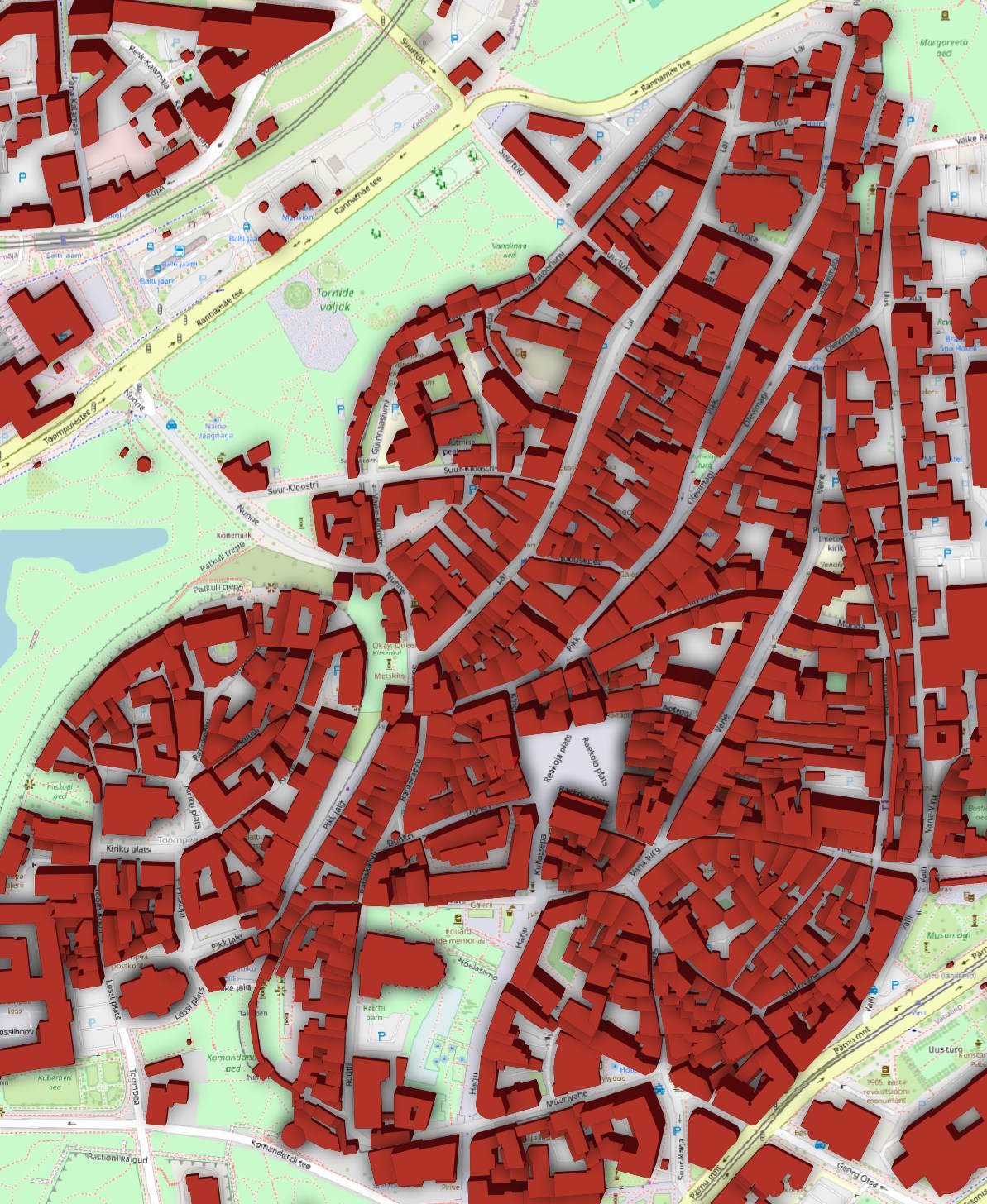
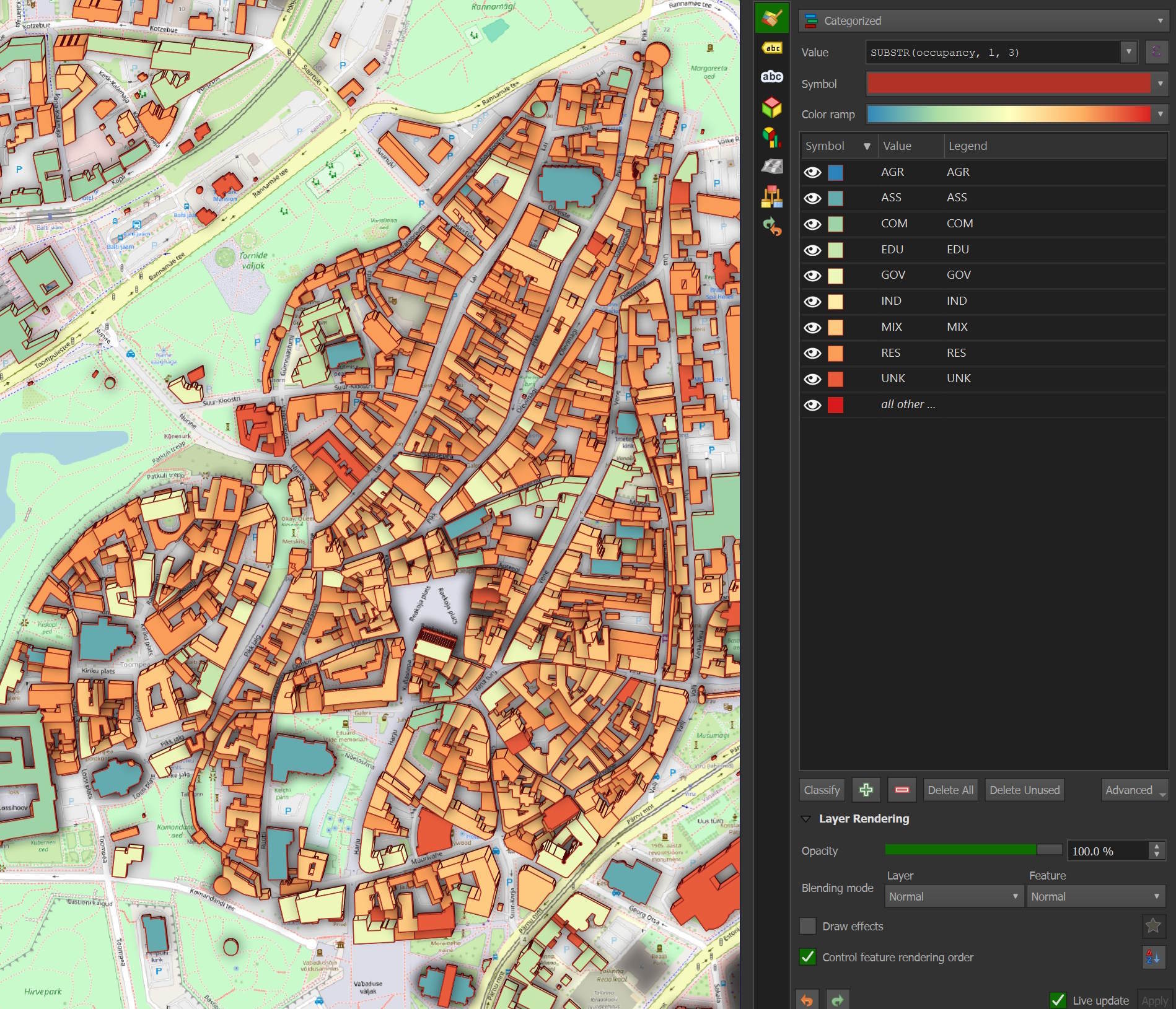
Below are the building use categories for each building in Tallinn's Old Town.
Building Sources
Google is the source for almost 60% of the building footprints. OSM accounts for 23% and Microsoft for 18%.
SELECT   COUNT(*),
         source
FROM     'building.*.parquet'
GROUP BY 2
ORDER BY 1 DESC;
┌──────────────┬───────────┐
│ count_star() │  source   │
│    int64     │  varchar  │
├──────────────┼───────────┤
│   1597737974 │ Google    │
│    612804756 │ OSM       │
│    482668539 │ Microsoft │
└──────────────┴───────────┘
OSM had 657M buildings in its dataset a few weeks ago so its interesting to see some ~45M of its buildings haven't made it into OBM.
Below I've highlighted the most common source for each H3 hexagon at zoom level 5.
CREATE OR REPLACE TABLE h3_5s AS
    WITH b AS (
        WITH a AS (
            SELECT   H3_LATLNG_TO_CELL(bbox.ymin,
                                       bbox.xmin,
                                       5) h3_5,
                     source,
                     COUNT(*) num_recs
            FROM     'building.*.parquet'
            GROUP BY 1, 2
        )
        SELECT *,
               ROW_NUMBER() OVER (PARTITION BY h3_5
                                  ORDER BY     num_recs DESC) AS rn
        FROM   a
    )
    FROM     b
    WHERE    rn = 1
    ORDER BY num_recs DESC;

COPY (
    SELECT geom: H3_CELL_TO_BOUNDARY_WKT(h3_5)::GEOMETRY,
           source
    FROM   h3_5s
    WHERE  ST_XMIN(geom::GEOMETRY) BETWEEN -179 AND 179
    AND    ST_XMAX(geom::GEOMETRY) BETWEEN -179 AND 179
) TO 'obm.top_sources.parquet' (
    FORMAT 'PARQUET',
    CODEC  'ZSTD',
    COMPRESSION_LEVEL 22,
    ROW_GROUP_SIZE 15000);
Microsoft is red, Google is green and OSM is yellow.
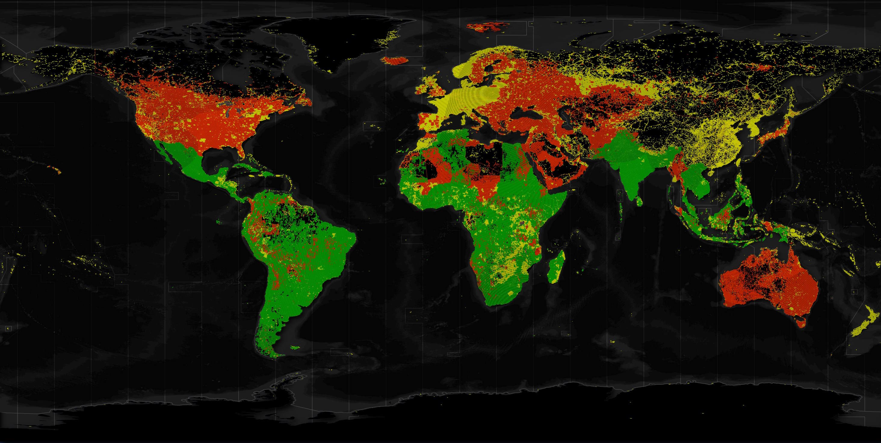
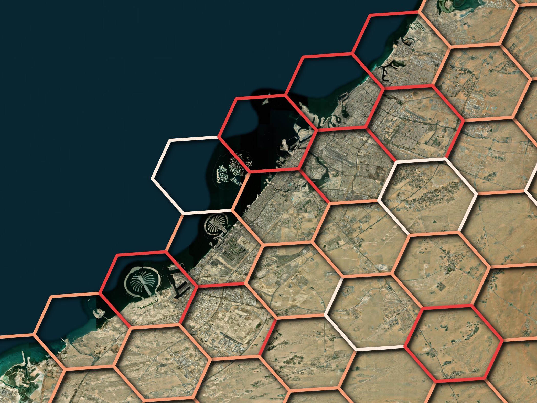
For spatial context, you'd only need a dozen or so of these zoom level 5 hexagons to cover Dubai's urban areas.
Building Heights
Both building height and/or the number of stories are contained within the height field. In some cases, ranges instead of absolute values are used. The field has the ability to express how many stories below ground a building extends as well. The "Building height" section in the paper goes into detail.
Below are the building counts by the initial height prefix and if the multiple measurements delimiter is present.
SELECT   prefix:        SPLIT(height, ':')[1],
         multi:         height LIKE '%+%',
         num_buildings: COUNT(*)
FROM     'building.*.parquet'
GROUP BY 1, 2
ORDER BY 3 DESC;
┌─────────┬─────────┬───────────────┐
│ prefix  │  multi  │ num_buildings │
│ varchar │ boolean │     int64     │
├─────────┼─────────┼───────────────┤
│ HBET    │ false   │    1879363563 │
│ NULL    │ NULL    │     667500586 │
│ HHT     │ false   │     114324028 │
│ H       │ false   │      27654116 │
│ H       │ true    │       4360694 │
│ HBEX    │ false   │          8036 │
│ HBEX    │ true    │           246 │
└─────────┴─────────┴───────────────┘
~25% of the buildings in this dataset don't have any height data.
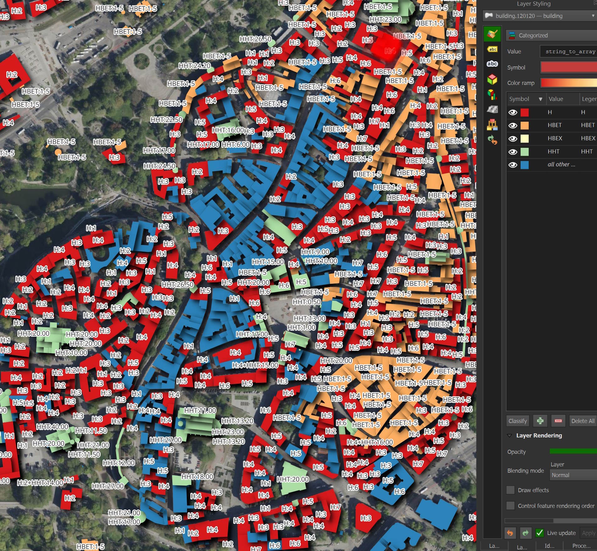
Below I've colour-coded the buildings in Tallinn's Old Town by their height prefix. The 'H' records in red contain the number of stories, the 'HBET' records in orange contain a range of stories, the 'HHT' records in light green contain the height in meters and the blue buildings have no height information.
Below are an example of combination values, delimited by a plus sign.
.maxrows 10

SELECT   height,
         COUNT(*)
FROM     'building.*.parquet'
WHERE    height LIKE '%+%'
GROUP BY 1
ORDER BY 2 DESC;
┌───────────────────────┬──────────────┐
│        height         │ count_star() │
│        varchar        │    int64     │
├───────────────────────┼──────────────┤
│ H:1+HHT:3.50          │       903295 │
│ H:2+HHT:7.00          │       395789 │
│ H:1+HHT:3.00          │       261288 │
│ H:2+HHT:6.00          │       136564 │
│ H:1+HHT:4.00          │       115217 │
│ H:2+HBEX:1            │        67691 │
│ H:1+HBEX:1            │        59680 │
│ H:1+HHT:5.00          │        51128 │
│ H:1+HHT:2.80          │        50296 │
│ H:2+HHT:8.00          │        48202 │
│ H:1+HHT:3.30          │        48074 │
│ H:1+HHT:3.40          │        47996 │
│ H:1+HHT:3.60          │        47382 │
│ H:3+HBEX:1            │        46986 │
│ H:1+HHT:3.20          │        43824 │
│ H:1+HHT:3.70          │        43422 │
│ H:1+HHT:3.80          │        40676 │
│ H:1+HHT:3.10          │        39174 │
│ H:3+HHT:9.00          │        38437 │
│ H:1+HHT:6.00          │        37171 │
│      ·                │            · │
│      ·                │            · │
│      ·                │            · │
│ H:2+HBEX:1+HHT:7.40   │            1 │
│ H:33+HHT:10.00        │            1 │
│ H:17+HBEX:1+HHT:49.60 │            1 │
│ H:15+HHT:4.80         │            1 │
│ H:15+HHT:71.50        │            1 │
│ H:1+HHT:15.51         │            1 │
│ H:42+HHT:136.55       │            1 │
│ H:60+HHT:239.12       │            1 │
│ H:53+HHT:229.00       │            1 │
│ H:39+HHT:98.00        │            1 │
│ H:8+HHT:2.90          │            1 │
│ H:35+HHT:82.00        │            1 │
│ H:7+HHT:12.20         │            1 │
│ H:4+HBEX:1+HHT:13.50  │            1 │
│ H:25+HHT:96.36        │            1 │
│ H:3+HBEX:1+HHT:10.55  │            1 │
│ H:32+HHT:142.00       │            1 │
│ H:43+HHT:147.70       │            1 │
│ H:11+HHT:35.09        │            1 │
│ H:65+HHT:258.00       │            1 │
├───────────────────────┴──────────────┤
│ 22423 rows (40 shown)      2 columns │
└──────────────────────────────────────┘
It would be nice to have separate columns for height in meters and stories both going above and below ground. I'll have to analyse this column further to figure out how complex that task would be.
Canadian Coverage
I'll download a rough outline of Canada's provinces and territories in GeoJSON format. I'll then convert it into GPKG as GPKG files require less syntax to work with in DuckDB.
$ wget -c https://gist.github.com/Thiago4breu/6ba01976161aa0be65e0a289412dc54c/raw/8ec57d8317a2abe5bae18e5fd86f777fab649f84/canada-provinces.geojson
$ ogr2ogr \
    -f GPKG \
    canada-provinces.gpkg \
    canada-provinces.geojson
$ ~/duckdb
CREATE OR REPLACE TABLE canada AS
    FROM ST_READ('canada-provinces.gpkg');

SELECT    COUNT(*)
FROM      'building.*.parquet' b
LEFT JOIN canada c ON ST_COVEREDBY(b.geometry, c.geom)
WHERE     c.name IS NOT NULL;
The above returned a count of 13,239,095 Canadian buildings in OBM.
For comparison, the ODB dataset I reviewed last month contains 14.4M buildings in Canada, PSC has 13.7M, TUM has 13.4M and the Layercake Project, which produces weekly exports of OSM data into Parquet and hosts via Cloudflare's CDN, has 7.8M Canadian buildings.
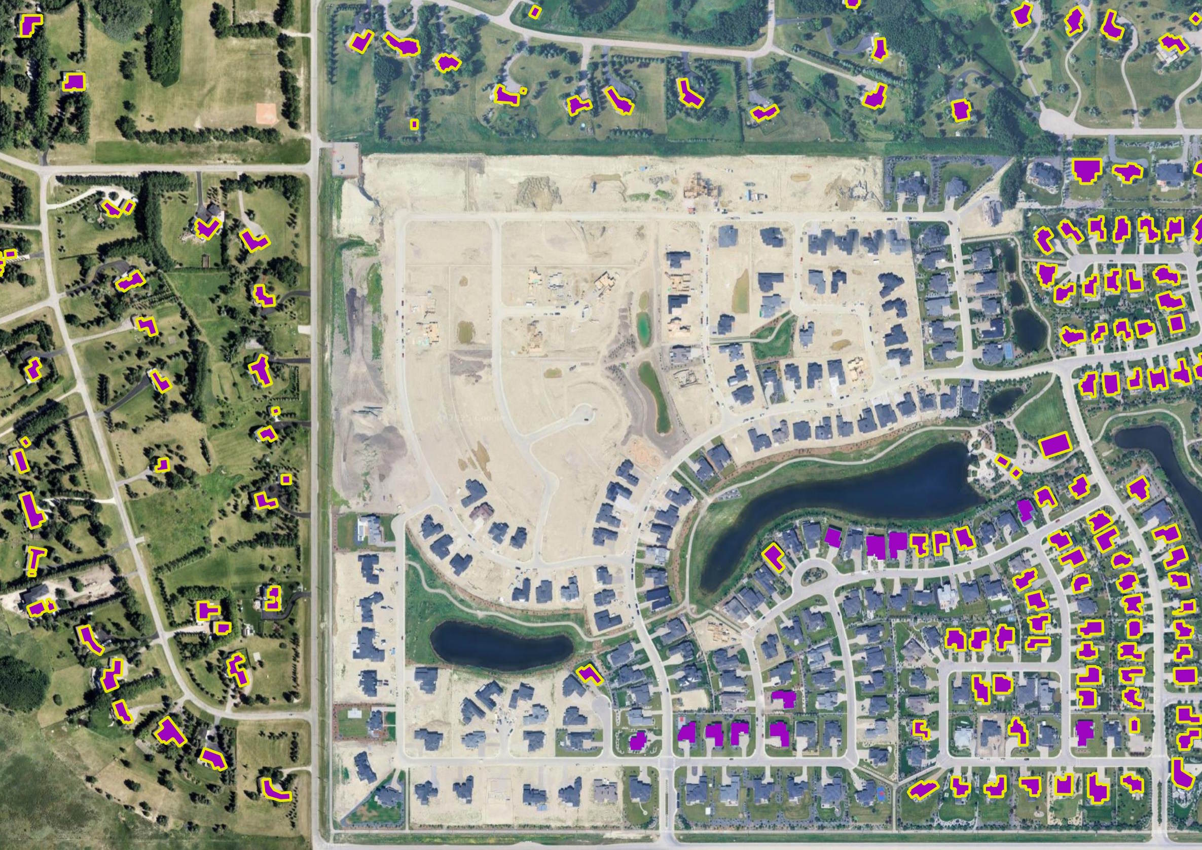
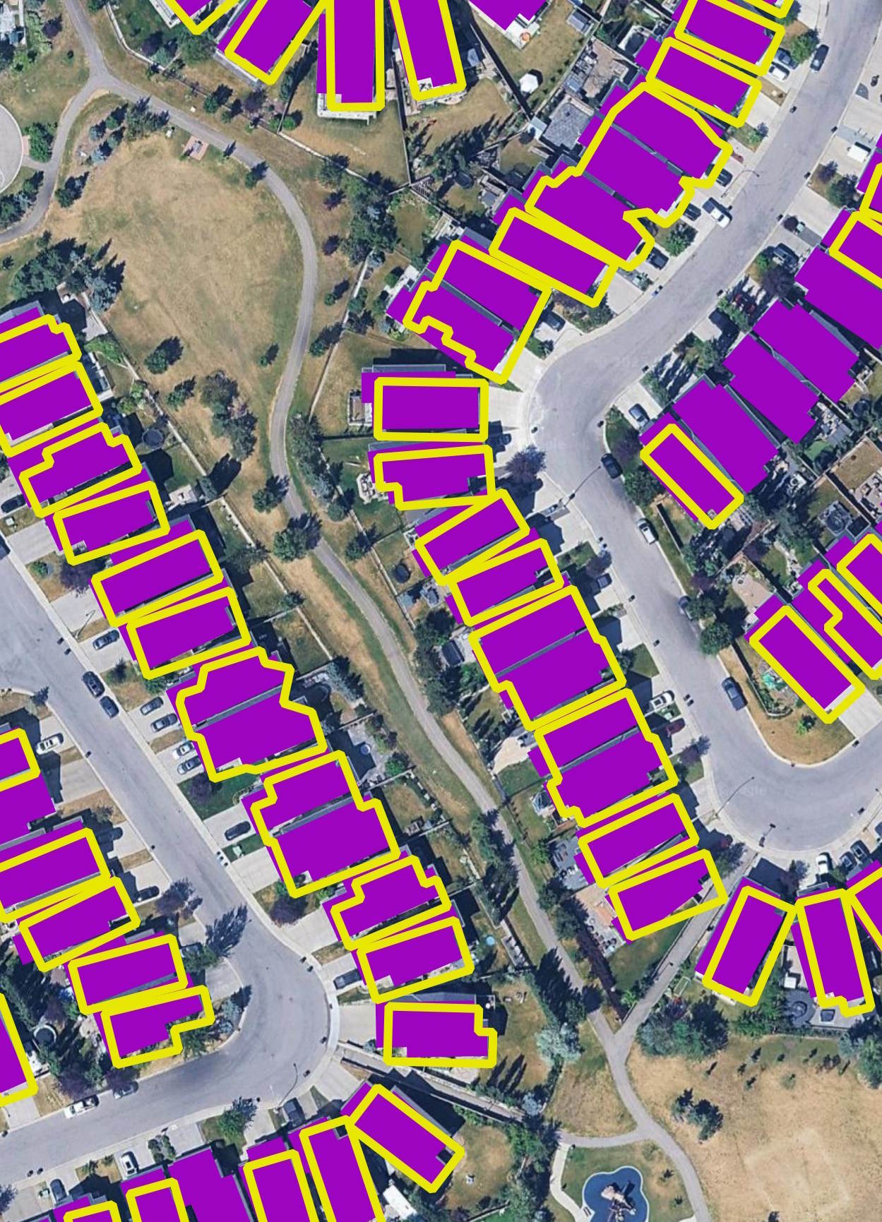
Below on top of Google's Satellite Map in yellow is OBM and in purple is Overture's October building footprints for South East Calgary. There are several areas where OBM has gaps in its coverage.
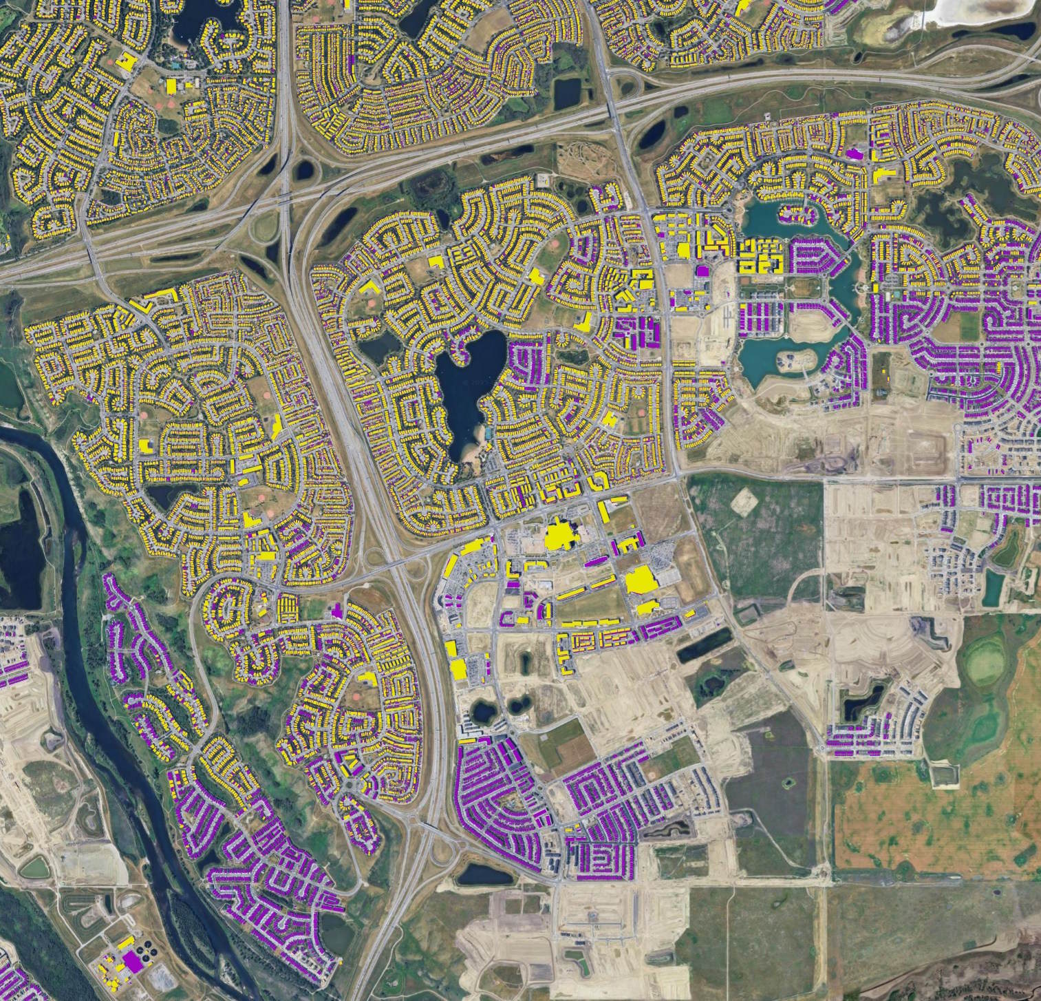
With that said, cities like Calgary are growing fast and new neighbourhoods can be waiting a while before they appear in any public datasets.
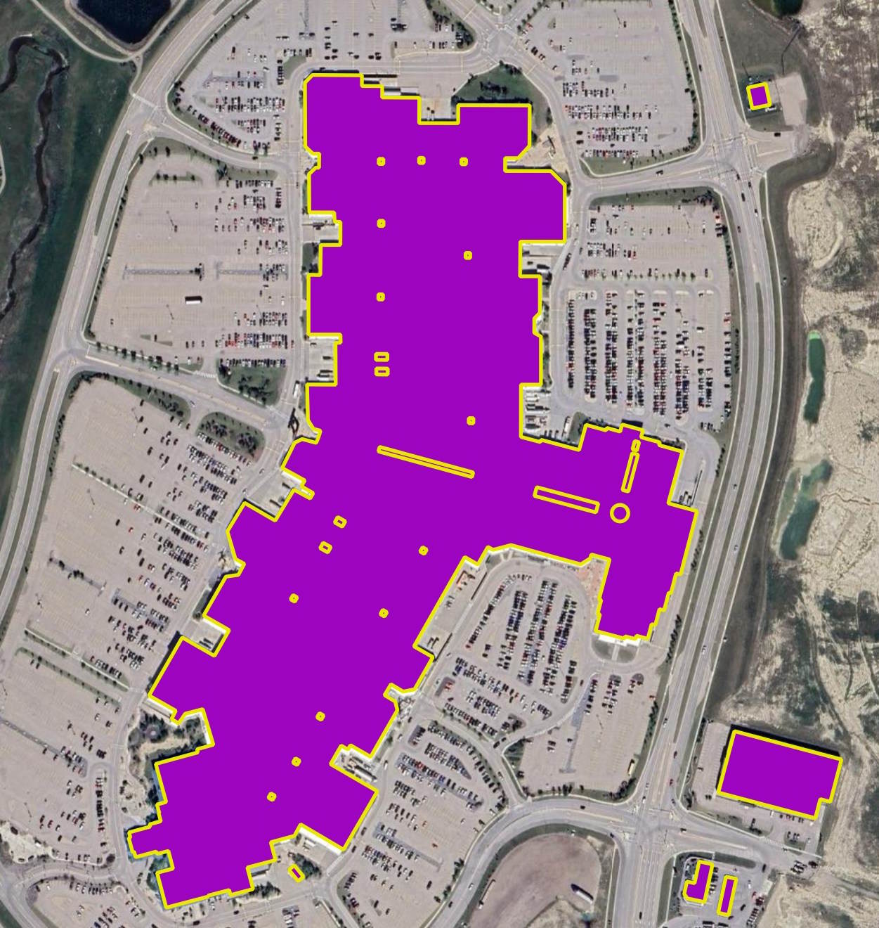
I spotted a few cases where a OBM building footprint will cover two or three properties.
This Mall, just north of Calgary's Airport, has ODM building footprints on top of one another.
For reference, Overture's October release contains 13,453,441 buildings for Canada.
SELECT    COUNT(*)
FROM      's3://overturemaps-us-west-2/release/2025-10-22.0/theme=buildings/type=building/part-000*.parquet' b
LEFT JOIN canada c ON ST_COVEREDBY(ST_POINT(bbox.xmin,
                                            bbox.ymin),
                                   c.geom)
WHERE     c.name IS NOT NULL;
Note: Overture has 236 Parquet files for its building footprints dataset. If I scan all of those files, the query above will exhaust my system's RAM capacity. So to get around this, the URL glob limits the query to just the first 100 Parquet files. The Parquet files are spatially sorted so Canada's data should usually live in the lower file numbers.