The United Nations (UN) believes there are 4B buildings on Earth. This week, a dataset called "GlobalBuildingAtlas" (GBA) was published by researchers at the Technical University of Munich (TUM) that attempts to estimate this number at being closer to 2.75B.
GBA is broken up into two datasets. The first is a 1.1 TB, level-of-detail 1 (LoD1) dataset made up of 922 uncompressed GeoJSON files. I spent the last few days downloading these and converting them into 210 GB of Parquet. These are now being hosted on AWS S3 thanks to the kind generosity of Source Cooperative and Taylor Geospatial Engine.
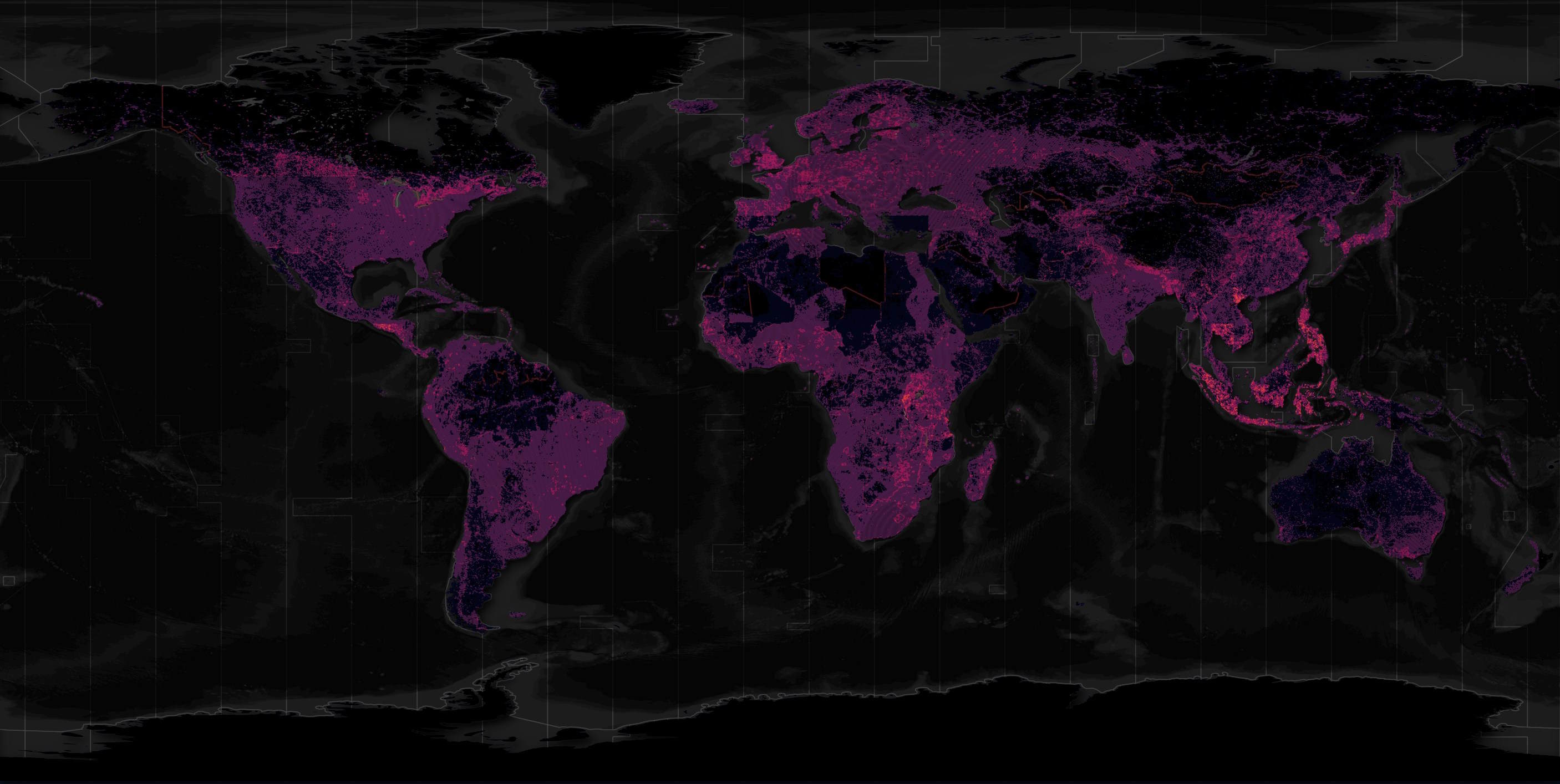
Below is a heatmap of this dataset.
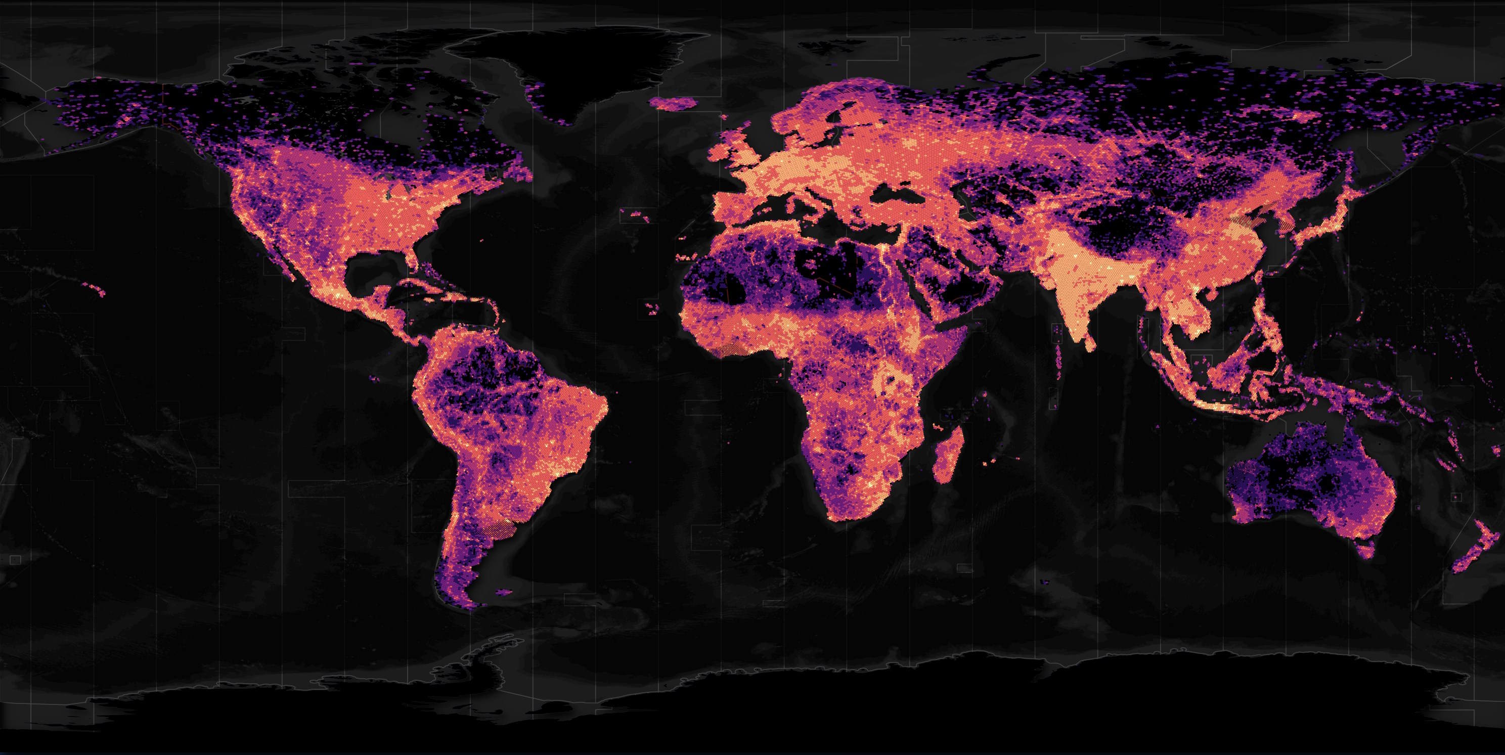
The above basemap is mostly made up of vector data from Natural Earth and Overture.
The second "Height" dataset is made up of 35 TB of raster height maps. Given the LoD1 files already contain building heights and downloading 35 TB off of TUM's servers will likely take months, I'll just show an individual raster in this post rather than run any dataset-wide operations on this dataset.
Parts of these datasets were developed by running open source (code, not imagery or weights) deep learning models on Planet Labs' satellite imagery. Planet Labs operate several constellations totalling hundreds of satellites in low earth orbit. They capture images of the entire Earth's landmasses every day.
In this post, I'll walk through loading the LoD1 data from S3 into QGIS, describe the ETL process I ran to build the Parquet version of this dataset and discuss some observations of the footprints themselves.
My Workstation
I'm using a 5.7 GHz AMD Ryzen 9 9950X CPU. It has 16 cores and 32 threads and 1.2 MB of L1, 16 MB of L2 and 64 MB of L3 cache. It has a liquid cooler attached and is housed in a spacious, full-sized Cooler Master HAF 700 computer case.
The system has 96 GB of DDR5 RAM clocked at 4,800 MT/s and a 5th-generation, Crucial T700 4 TB NVMe M.2 SSD which can read at speeds up to 12,400 MB/s. There is a heatsink on the SSD to help keep its temperature down. This is my system's C drive.
The system is powered by a 1,200-watt, fully modular Corsair Power Supply and is sat on an ASRock X870E Nova 90 Motherboard.
I'm running Ubuntu 24 LTS via Microsoft's Ubuntu for Windows on Windows 11 Pro. In case you're wondering why I don't run a Linux-based desktop as my primary work environment, I'm still using an Nvidia GTX 1080 GPU which has better driver support on Windows and ArcGIS Pro only supports Windows natively.
Installing Prerequisites
I'll use Python 3.12.3 and a few other tools to help analyse the data in this post.
$ sudo add-apt-repository ppa:deadsnakes/ppa
$ sudo apt update
$ sudo apt install \
    exiftool \
    jq \
    python3-pip \
    python3.12-venv
I'll be using JSON Convert (jc) to convert the output of various CLI tools into JSON.
$ wget https://github.com/kellyjonbrazil/jc/releases/download/v1.25.2/jc_1.25.2-1_amd64.deb
$ sudo dpkg -i jc_1.25.2-1_amd64.deb
I'll use a Parquet debugging tool I've been working on to see how much space each column takes up in one of the Parquet files.
$ git clone https://github.com/marklit/pqview \
    ~/pqview

$ python3 -m venv ~/.pqview
$ source ~/.pqview/bin/activate
$ python3 -m pip install \
          -r ~/pqview/requirements.txt
I'll use DuckDB, along with its H3, JSON, Lindel, Parquet and Spatial extensions, in this post.
$ cd ~
$ wget -c https://github.com/duckdb/duckdb/releases/download/v1.3.2/duckdb_cli-linux-amd64.zip
$ unzip -j duckdb_cli-linux-amd64.zip
$ chmod +x duckdb
$ ~/duckdb
INSTALL h3 FROM community;
INSTALL lindel FROM community;
INSTALL json;
INSTALL parquet;
INSTALL spatial;
I'll set up DuckDB to load every installed extension each time it launches.
$ vi ~/.duckdbrc
.timer on
.width 180
LOAD h3;
LOAD lindel;
LOAD json;
LOAD parquet;
LOAD spatial;
The maps in this post were rendered with QGIS version 3.44. QGIS is a desktop application that runs on Windows, macOS and Linux. The application has grown in popularity in recent years and has ~15M application launches from users all around the world each month.
Downloading the Buildings
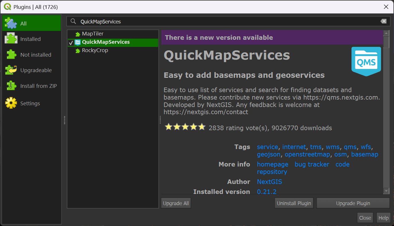
In QGIS, click the "Plugins" Menu and then the "Manage and Install Plugins" item. Click the "All" filter in the top left of the dialog and then search for "QuickMapServices". Click to install or upgrade the plugin in the bottom right of the dialog.
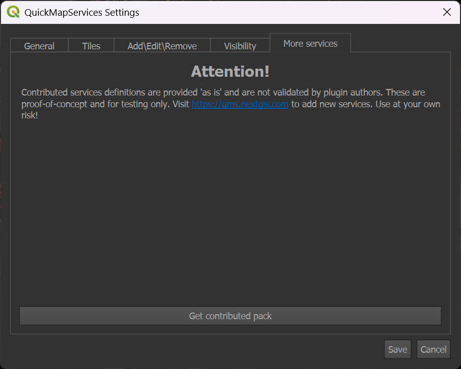
Click the "Web" Menu, then "QuickMapServices" and then the "Settings" item. Click the "More Services" tab at the top of the dialog. Click the "Get contributed pack" button.
In the "Web" menu under "QuickMapServices" you should now see the list of several basemap providers.
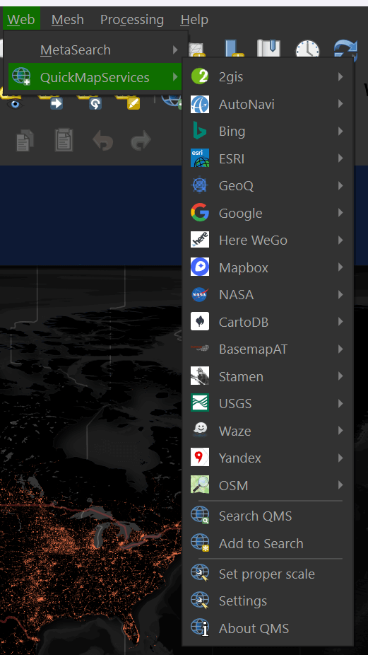
Select "OSM" and then "OSM Standard" to add a world map to your scene.
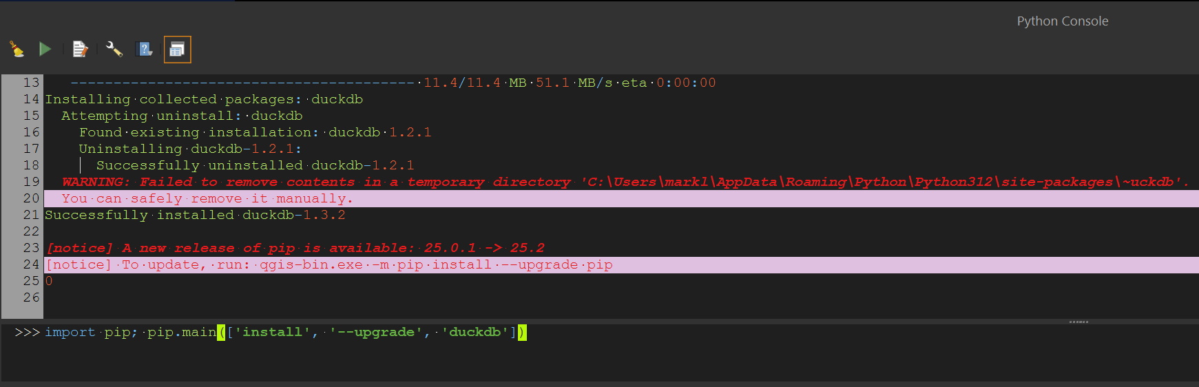
Under the "Plugins" menu, select "Python Console". Paste in the following line of Python. It'll ensure you've got the latest version of DuckDB installed in QGIS' Python Environment.
import pip; pip.main(['install', '--upgrade', 'duckdb'])
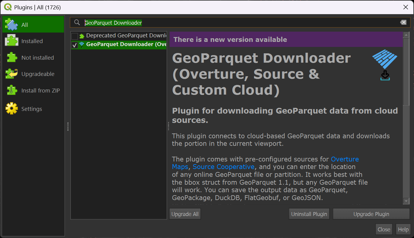
In QGIS, click the "Plugins" Menu and then the "Manage and Install Plugins" item. Click the "All" filter in the top left of the dialog and then search for "GeoParquet Downloader". Click to install or upgrade the plugin in the bottom right of the dialog.
Zoom into a city of interest somewhere in the world. It's important to make sure you're not looking at an area larger than a major city as the viewport will set the boundaries for how much data will be downloaded.
If you can see the whole earth, GeoParquet Downloader will end up downloading 210 GB of data. Downloading only a city's worth of data will likely only need a few MB of data.
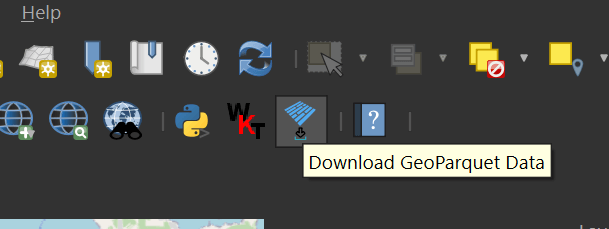
In your toolbar, click on the GeoParquet Downloader icon. It's the one with blue, rotated rectangles.
Click the "Custom URL" option and paste the following URL in.
s3://us-west-2.opendata.source.coop/tge-labs/globalbuildingatlas-lod1/*.parquet
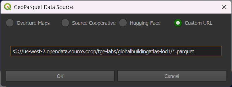
Hit "OK". You'll be prompted to save a Parquet file onto your computer. Once you've done so, the GBA data for the area in your map should appear shortly afterword.
Once the buildings have loaded, select the layer styling for the downloaded buildings layer. The combo box at the top of the styling panel should be switched from "Single Symbol" to "2.5D".
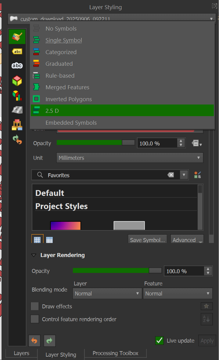
In the "Height" field, change it to the following expression:
min("height", 1) / 50000
You should now see a 2.5D representation of the buildings you downloaded.
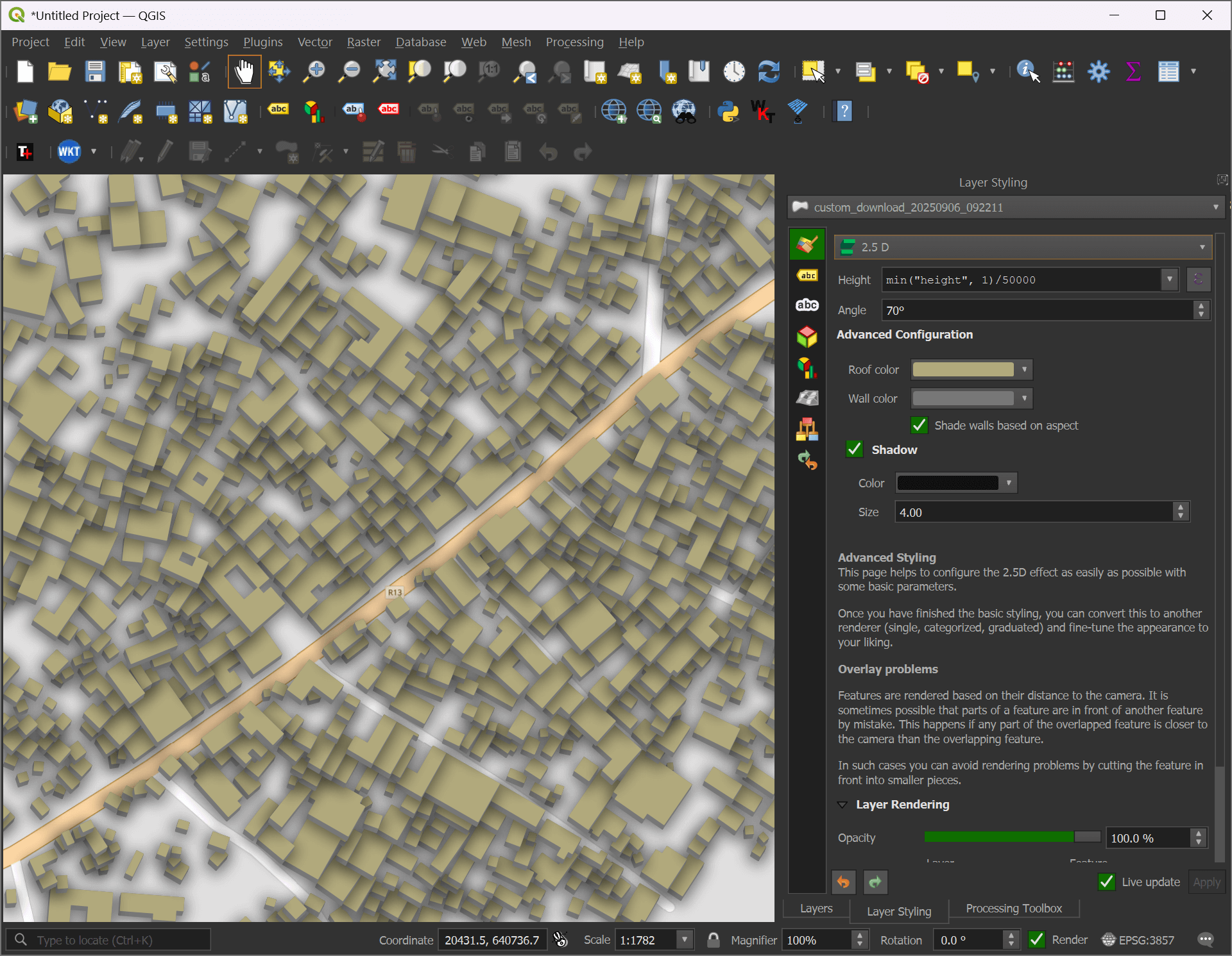
There is an "Identify Features" icon in the toolbar.
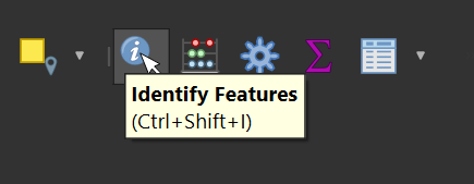
This tool lets you select any building and bring up its metadata.
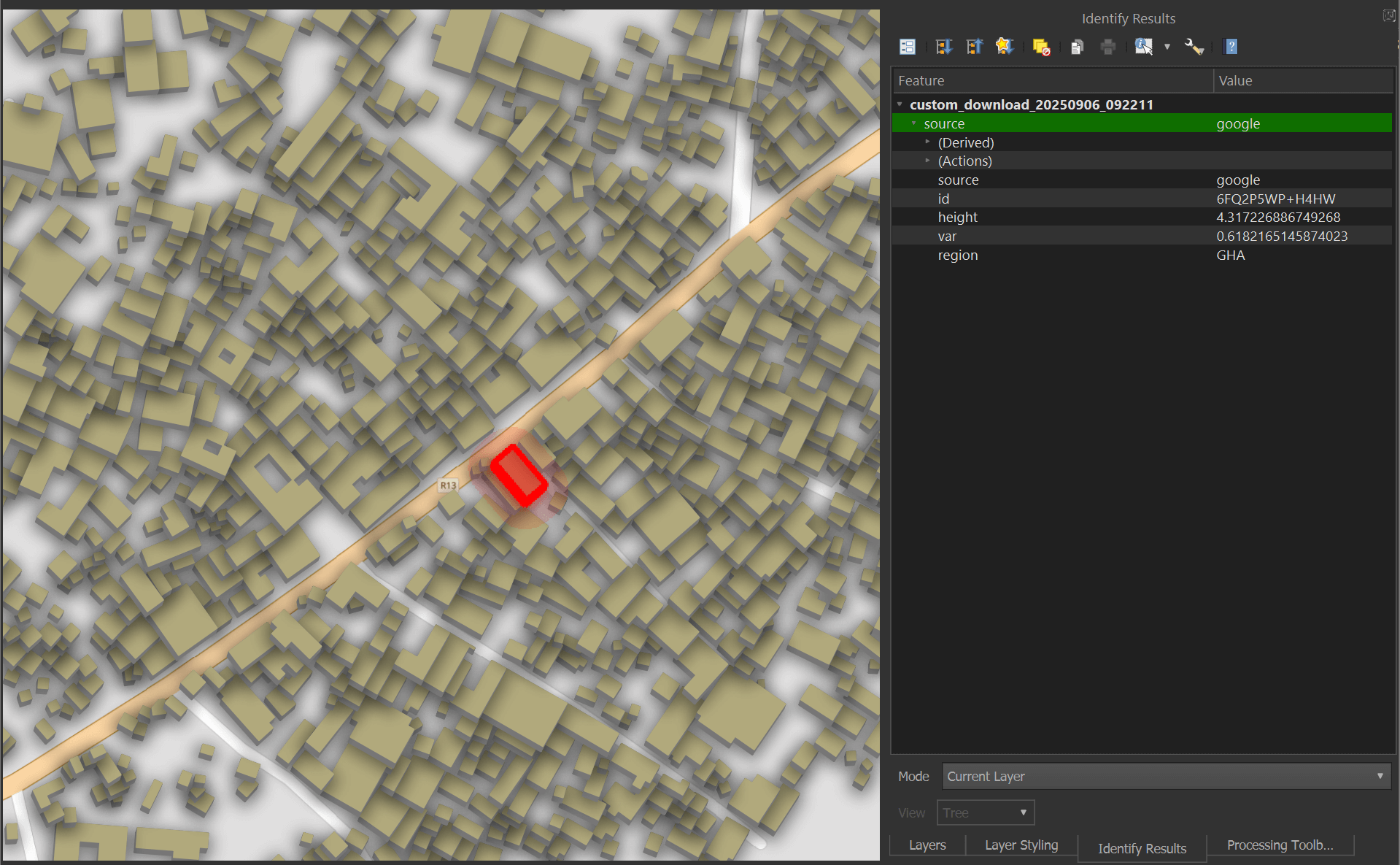
The Parquet file you saved can also be read via DuckDB and even dropped into Esri's ArcGIS Pro 3.5 or newer if you have it installed on your machine.
The LoD1 URLs
Below I'll discuss how I turned the 1.1 TB of GeoJSON into Parquet. These steps don't need to be repeated as the resulting files are now on S3.
I first set up a working folder on a partition that had at least 600 GB of free space.
$ mkdir -p ~/tum/stats
$ cd ~/tum
I built a 922-line list of URLs for the LoD1 dataset. They're available from this gist and I have them saved as manifest.lod.txt. Below are a few lines from this file.
$ head -n5 manifest.lod.txt
https://dataserv.ub.tum.de/s/m1782307/download?path=%2FLoD1%2Fafrica&files=e000_n10_e005_n05.geojson
https://dataserv.ub.tum.de/s/m1782307/download?path=%2FLoD1%2Fafrica&files=e000_n15_e005_n10.geojson
https://dataserv.ub.tum.de/s/m1782307/download?path=%2FLoD1%2Fafrica&files=e000_n20_e005_n15.geojson
https://dataserv.ub.tum.de/s/m1782307/download?path=%2FLoD1%2Fafrica&files=e000_n25_e005_n20.geojson
https://dataserv.ub.tum.de/s/m1782307/download?path=%2FLoD1%2Fafrica&files=e000_n30_e005_n25.geojson
I collected file size data for these URLs from TUM's server.
$ touch lods1.json && rm lods1.json

$ for URL in `cat manifest.txt`; do
    echo $URL
    curl -sI "$URL" | jc --kv >> lods1.json
  done
I then used Python to clean up some of the output and make it easier to analyse.
$ python3
import json
from   urllib.parse import unquote


urls  = [x.strip()     for x in open('manifest.lod.txt', 'r').readlines()]
resps = [json.loads(x) for x in open('lods1.json', 'r').readlines()]

for num, resp in enumerate(resps):
    resp['content_length'] = int(resp['content-length'])
    resp['http_code']      = [int(x.split(' ')[-1])
                              for x in resp.keys()
                              if x.startswith('HTTP/2')][0]

    resp['filename'] = resp['content-disposition']\
                            .split('filename=')[-1]\
                            .strip('"')
    resp['url']      = [x for x in urls if resp['filename'] in x][0]
    resp['folder']   = unquote(resp['url']
                                .split('path=')[-1]
                                .split('&')[0])

    resps[num] = resp

open('lods1.enriched.json', 'w')\
    .write('\n'.join(json.dumps(x) for x in resps))
There were 922 HTTP 200 responses from the above crawl. One for every URL in the manifest.
$ ~/duckdb
SELECT   http_code,
         COUNT(*)
FROM     'lods1.enriched.json'
GROUP BY 1;
┌───────────┬──────────────┐
│ http_code │ count_star() │
│   int64   │    int64     │
├───────────┼──────────────┤
│    200    │     922      │
└───────────┴──────────────┘
This is the number of GB each region of the world contains on TUM's servers. Note, this is all uncompressed GeoJSON.
SELECT   folder,
         (SUM(content_length) / 1024 ** 3)::INT AS GB
FROM     'lods1.enriched.json'
GROUP BY 1
ORDER BY 2 DESC;
┌────────────────────┬───────┐
│       folder       │  GB   │
│      varchar       │ int32 │
├────────────────────┼───────┤
│ /LoD1/asiawest     │   388 │
│ /LoD1/africa       │   294 │
│ /LoD1/europe       │   202 │
│ /LoD1/northamerica │   147 │
│ /LoD1/southamerica │   140 │
│ /LoD1/asiaeast     │   108 │
│ /LoD1/oceania      │    67 │
└────────────────────┴───────┘
These are the number of GeoJSON files that make up each region of the world.
SELECT   folder,
         COUNT(*) num_urls
FROM     'lods1.enriched.json'
GROUP BY 1
ORDER BY 2 DESC;
┌────────────────────┬──────────┐
│       folder       │ num_urls │
│      varchar       │  int64   │
├────────────────────┼──────────┤
│ /LoD1/northamerica │      179 │
│ /LoD1/africa       │      176 │
│ /LoD1/asiawest     │      130 │
│ /LoD1/asiaeast     │      128 │
│ /LoD1/oceania      │      114 │
│ /LoD1/southamerica │      101 │
│ /LoD1/europe       │       94 │
└────────────────────┴──────────┘
These are the smallest and largest files in the LoD1 dataset.
SELECT   content_length,
         folder,
         filename
FROM     'lods1.enriched.json'
ORDER BY content_length;
┌────────────────┬────────────────────┬───────────────────────────┐
│ content_length │       folder       │         filename          │
│     int64      │      varchar       │          varchar          │
├────────────────┼────────────────────┼───────────────────────────┤
│            674 │ /LoD1/asiaeast     │ e135_n25_e140_n20.geojson │
│            677 │ /LoD1/asiaeast     │ e170_n75_e175_n70.geojson │
│           2137 │ /LoD1/northamerica │ w050_n60_w045_n55.geojson │
│           3437 │ /LoD1/asiawest     │ e095_n70_e100_n65.geojson │
│           5746 │ /LoD1/northamerica │ w105_n65_w100_n60.geojson │
│           6913 │ /LoD1/northamerica │ w145_n60_w140_n55.geojson │
│          11094 │ /LoD1/southamerica │ w030_s20_w025_s25.geojson │
│          12586 │ /LoD1/northamerica │ w125_n75_w120_n70.geojson │
│          14778 │ /LoD1/northamerica │ w075_n60_w070_n55.geojson │
│          15223 │ /LoD1/oceania      │ e165_n05_e170_n00.geojson │
│          18611 │ /LoD1/asiaeast     │ e150_n75_e155_n70.geojson │
│          20510 │ /LoD1/oceania      │ e115_s15_e120_s20.geojson │
│          23356 │ /LoD1/asiaeast     │ e115_n75_e120_n70.geojson │
│          27109 │ /LoD1/northamerica │ w150_n60_w145_n55.geojson │
│          29734 │ /LoD1/asiawest     │ e085_n75_e090_n70.geojson │
│          31258 │ /LoD1/oceania      │ e065_s45_e070_s50.geojson │
│          32752 │ /LoD1/asiaeast     │ e160_n55_e165_n50.geojson │
│          32891 │ /LoD1/northamerica │ w170_n20_w165_n15.geojson │
│          33177 │ /LoD1/europe       │ e055_n75_e060_n70.geojson │
│          34303 │ /LoD1/northamerica │ w065_n65_w060_n60.geojson │
│            ·   │      ·             │             ·             │
│            ·   │      ·             │             ·             │
│            ·   │      ·             │             ·             │
│    12115126130 │ /LoD1/europe       │ e005_n50_e010_n45.geojson │
│    12663234796 │ /LoD1/asiawest     │ e090_n25_e095_n20.geojson │
│    12907517141 │ /LoD1/africa       │ e030_n05_e035_n00.geojson │
│    13682576090 │ /LoD1/northamerica │ w100_n20_w095_n15.geojson │
│    13778082922 │ /LoD1/asiawest     │ e075_n20_e080_n15.geojson │
│    13858487472 │ /LoD1/asiawest     │ e070_n30_e075_n25.geojson │
│    14316795070 │ /LoD1/asiawest     │ e075_n25_e080_n20.geojson │
│    14440822865 │ /LoD1/asiawest     │ e105_n15_e110_n10.geojson │
│    14459258848 │ /LoD1/southamerica │ w050_s20_w045_s25.geojson │
│    14558343630 │ /LoD1/asiawest     │ e080_n25_e085_n20.geojson │
│    15756826807 │ /LoD1/europe       │ e005_n55_e010_n50.geojson │
│    15986484228 │ /LoD1/oceania      │ e105_s05_e110_s10.geojson │
│    16830813690 │ /LoD1/asiawest     │ e070_n25_e075_n20.geojson │
│    18731290715 │ /LoD1/oceania      │ e110_s05_e115_s10.geojson │
│    22094633389 │ /LoD1/asiawest     │ e085_n30_e090_n25.geojson │
│    24040590951 │ /LoD1/asiawest     │ e070_n35_e075_n30.geojson │
│    24784041081 │ /LoD1/asiawest     │ e075_n15_e080_n10.geojson │
│    27418761453 │ /LoD1/asiawest     │ e085_n25_e090_n20.geojson │
│    31113223192 │ /LoD1/asiawest     │ e080_n30_e085_n25.geojson │
│    31830016696 │ /LoD1/asiawest     │ e075_n30_e080_n25.geojson │
├────────────────┴────────────────────┴───────────────────────────┤
│ 922 rows (40 shown)                                   3 columns │
└─────────────────────────────────────────────────────────────────┘
Downloading GeoJSON
One day after I started downloading the GeoJSON files, the URLs were changed on TUM's server. I had to run the following script to produce a new list of URLs to download.
$ echo "SELECT 'https://dataserv.ub.tum.de/public.php/dav/files/m1782307/LoD1/'
                    || REPLACE(folder, '/LoD1/', '')
                    || '/'
                    || filename AS url
         FROM   'lods1.enriched.json'" \
    | ~/duckdb -csv -noheader \
    > manifest.lod.dav.txt
Below is the download script I used. Once a file was downloaded, it was compressed to preserve space on my machine. The files are downloaded in a random order and after each pass of the 922 URLs, any missing files not downloaded will be retried. I experienced several outages of TUMs server during this process so the retries came in handy.
$ while :
  do
      for LINE in `sort -R manifest.lod.dav.txt`; do
          GEOJSON=`echo "$LINE" | cut -d/ -f10`
          ZIPFILE="$GEOJSON.zip"

          if [ ! -f $ZIPFILE ]; then
              echo $LINE
              wget -c -O $GEOJSON "$LINE"

              LINE_COUNT=$(wc -l < $GEOJSON)

              if [ "$LINE_COUNT" -eq 0 ]; then
                  rm "$GEOJSON"
                  echo "$GEOJSON has zero lines. Sleeping for 3 minutes.."
                  sleep 180
              else
                  zip -9v "$ZIPFILE" "$GEOJSON"
                  rm "$GEOJSON"
              fi
          else
              echo "$ZIPFILE already exists, skipping.."
          fi
      done

      echo "Finished a pass of the manifest file. Sleeping for 5 minutes.."
      sleep 300
  done
The above took the better part of a week to complete. The 1.1 TB of uncompressed GeoJSON was compressed into 357 GB worth of ZIP files.
GeoJSON to Parquet
The following GeoJSON to Parquet script ran concurrently to the above download script. It extracts the GeoJSON file inside of any unprocessed ZIP file, converts its projection from EPSG:3857 to EPSG:4326, creates a bounding box and spatially sorts the dataset into a ZStandard-compressed Parquet file.
This script runs on a loop and looks for new files process during each run. The GeoJSON to Parquet process is pretty quick on my machine so this script spent a lot of time waiting for new ZIPs.
$ while :
  do
      for ZIPFILE in *.geojson.zip; do
          BASENAME=`echo "$ZIPFILE" | cut -f1 -d.`
          PQ_FILE="$BASENAME.parquet"

          if [ ! -f $PQ_FILE ]; then
              echo $BASENAME

              mkdir -p working
              rm working/* || true 2>/dev/null
              unzip $ZIPFILE -d working/
              FIRST=`ls working/*.geojson | head -n1`

              echo "COPY (
                        SELECT   * EXCLUDE (geom),
                                 ST_FLIPCOORDINATES(
                                      ST_TRANSFORM(geom,
                                                   'EPSG:3857',
                                                   'EPSG:4326')) geometry,
                                 {'xmin': ST_XMIN(ST_EXTENT(ST_FLIPCOORDINATES(
                                              ST_TRANSFORM(geom,
                                                           'EPSG:3857',
                                                           'EPSG:4326')))),
                                  'ymin': ST_YMIN(ST_EXTENT(ST_FLIPCOORDINATES(
                                              ST_TRANSFORM(geom,
                                                           'EPSG:3857',
                                                           'EPSG:4326')))),
                                  'xmax': ST_XMAX(ST_EXTENT(ST_FLIPCOORDINATES(
                                              ST_TRANSFORM(geom,
                                                           'EPSG:3857',
                                                           'EPSG:4326')))),
                                  'ymax': ST_YMAX(ST_EXTENT(ST_FLIPCOORDINATES(
                                              ST_TRANSFORM(geom,
                                                           'EPSG:3857',
                                                           'EPSG:4326'))))} AS bbox
                        FROM     ST_READ('$FIRST')
                        ORDER BY HILBERT_ENCODE([
                              ST_Y(ST_CENTROID(ST_FLIPCOORDINATES(
                                      ST_TRANSFORM(geom,
                                                   'EPSG:3857',
                                                   'EPSG:4326')))),
                              ST_X(ST_CENTROID(ST_FLIPCOORDINATES(
                                      ST_TRANSFORM(geom,
                                                   'EPSG:3857',
                                                   'EPSG:4326'))))]::double[2])
                    ) TO '$BASENAME.parquet' (
                        FORMAT            'PARQUET',
                        CODEC             'ZSTD',
                        COMPRESSION_LEVEL 22,
                        ROW_GROUP_SIZE    15000);" | ~/duckdb
          else
              echo "$PQ_FILE already exists, skipping.."
          fi
      done

      echo "Sleeping for 5 minutes.."
      sleep 300
  done
The above turned the 357 GB worth of ZIPs into 210 GB of Parquet.
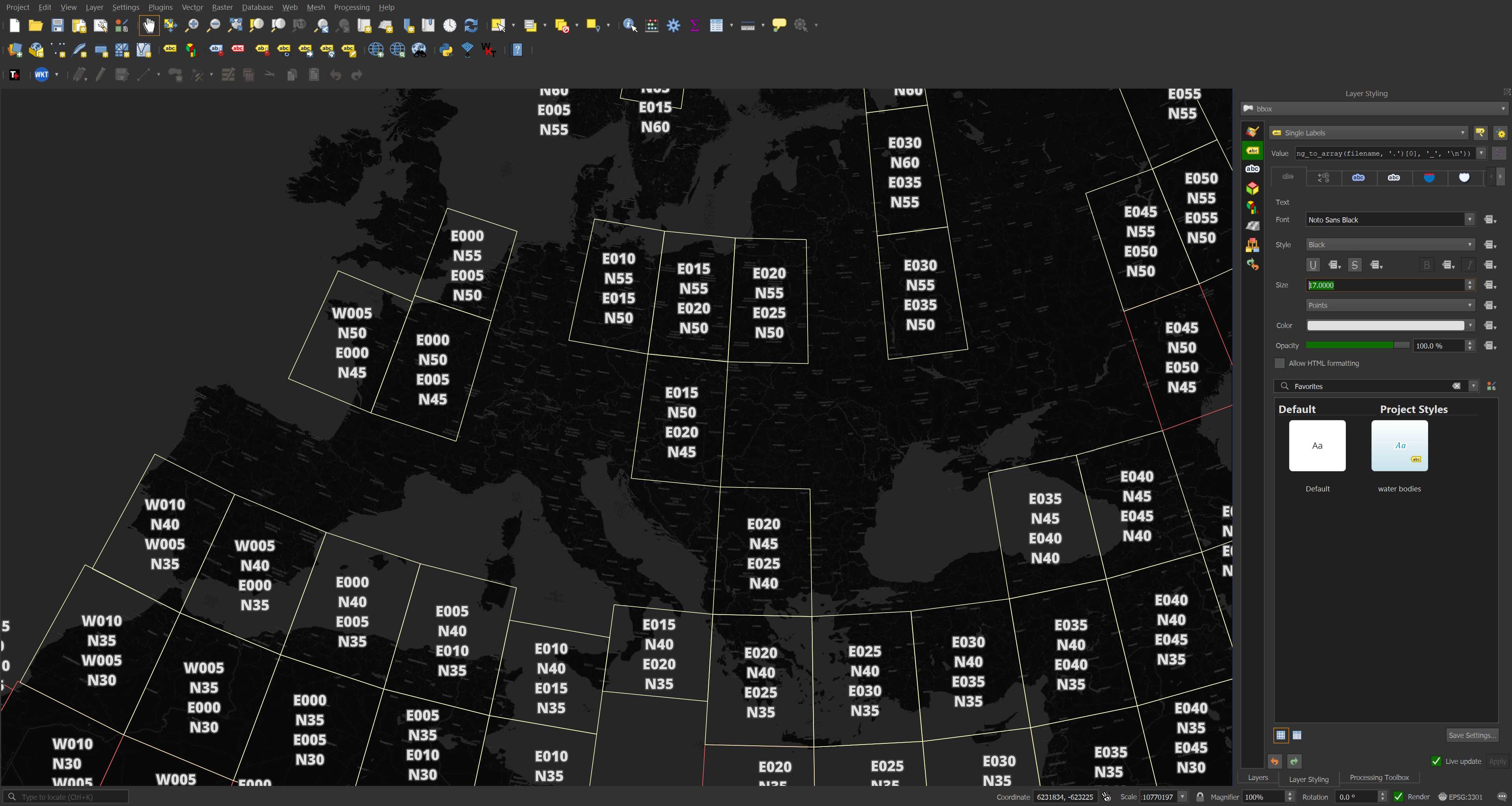
The base filenames of the Parquet files match their GeoJSON counterparts. These GeoJSON files used a e115_n45_e120_n40.geojson convention where the filename indicated where the contents were located.
Below I've rendered the footprints with their filenames formatted for clarity. This was run while the download script was still going so there are footprints missing in this screen shot. The basemap used is CARTO Dark.
$ ~/duckdb
COPY (
    WITH a AS (
        SELECT ST_XMIN(ST_EXTENT(geometry)) AS xmin,
               ST_YMIN(ST_EXTENT(geometry)) AS ymin,
               ST_XMAX(ST_EXTENT(geometry)) AS xmax,
               ST_YMAX(ST_EXTENT(geometry)) AS ymax,
               filename
        FROM   READ_PARQUET('*.parquet', filename=true)
    )
    SELECT   filename,
             ST_ASWKB({'min_x': MIN(xmin),
                       'min_y': MIN(ymin),
                       'max_x': MAX(xmax),
                       'max_y': MAX(ymax)}::BOX_2D::GEOMETRY) AS geometry,
             COUNT(*) num_buildings
    FROM     a
    GROUP BY filename
    ORDER BY filename
) TO 'stats/bbox.parquet' (
        FORMAT            'PARQUET',
        CODEC             'ZSTD',
        COMPRESSION_LEVEL 22,
        ROW_GROUP_SIZE    15000);
LoD1 Records
There are 2,747,186,815 records in this dataset with each record representing one building.
$ ~/duckdb
SELECT COUNT(*)
FROM   READ_PARQUET('*.parquet');
2747186815
For comparison, Overture's August release contains 2,539,170,484 buildings (~208M fewer).
$ ~/duckdb
SELECT COUNT(*)
FROM   READ_PARQUET('s3://overturemaps-us-west-2/release/2025-08-20.0/theme=buildings/type=building/*.parquet',
                    hive_partitioning=1);
2539170484
Below is an example LoD1 record.
$ echo "SELECT * EXCLUDE(bbox),
               bbox::JSON AS bbox
        FROM  READ_PARQUET('e000_n10_e005_n05.parquet')
        LIMIT 1" \
    | ~/duckdb -json \
    | jq -S .
[
  {
    "bbox": {
      "xmax": 0.00008150001546320158,
      "xmin": 0.0,
      "ymax": 7.993254849391249,
      "ymin": 7.993157996915336
    },
    "geometry": "POLYGON ((0.000052522233915 7.993254849391249, 0.000081500015463 7.993157996915336, 0 7.993181313497494, 0.000052522233915 7.993254849391249))",
    "height": 6.524652481079102,
    "id": "4538",
    "region": "GHA",
    "source": "ours2",
    "var": 0.7772102355957031
  }
]
Below I'll generate a heatmap of the records and render them in QGIS.
$ ~/duckdb stats/stats.duckdb
CREATE OR REPLACE TABLE h3_4_stats AS
    SELECT   H3_LATLNG_TO_CELL(
                bbox.ymin,
                bbox.xmin, 4) AS h3_4,
             COUNT(*) num_buildings
    FROM     READ_PARQUET('*.parquet')
    WHERE    bbox.xmin BETWEEN -178.5 AND 178.5
    GROUP BY 1;

COPY (
    SELECT ST_ASWKB(H3_CELL_TO_BOUNDARY_WKT(h3_4)::geometry) geometry,
           num_buildings
    FROM   h3_4_stats
) TO 'stats/h3_4_stats.parquet' (
        FORMAT 'PARQUET',
        CODEC  'ZSTD',
        COMPRESSION_LEVEL 22,
        ROW_GROUP_SIZE 15000);
Bounding Boxes
In the above rendering I've used the bounding box values instead of the underlying geometry. This produces results quicker. This is due to the values taking up less space and not needing as many transformations as the underlying geometry would.
Below is a pie chart showing how much space each column takes up in one of the Parquet files. The bbox.xmin and bbox.ymin fields are much smaller than the geometry field.
$ python3 ~/pqview/main.py \
    types --html \
    e000_n10_e005_n05.parquet \
    > stats/e000_n10_e005_n05.html
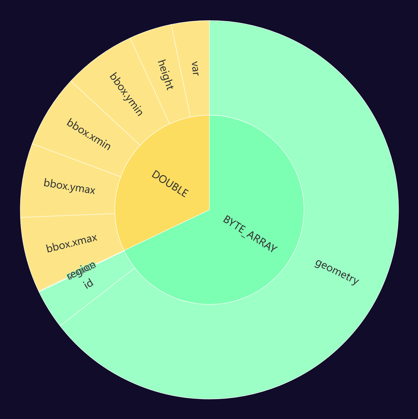
The GeoParquet Downloader Plugin for QGIS also uses these bounding boxes to download data quicker than it would if it had used the geometry field alone.
Data Sources
Below are the sources of data in GBA.
$ ~/duckdb
SELECT   COUNT(*),
         source
FROM     READ_PARQUET('*.parquet')
GROUP BY 2
ORDER BY 1 DESC;
┌──────────────┬──────────┐
│ count_star() │  source  │
│    int64     │ varchar  │
├──────────────┼──────────┤
│   1619713039 │ google   │
│    490593924 │ osm      │
│    432475081 │ ms       │
│    135815381 │ ours2    │
│     68589390 │ 3dglobfp │
└──────────────┴──────────┘
Google's 2023 Open Buildings data is the most used. The OSM data is from 2025 but I'm not sure which month and day. Microsoft Building Footprints is from 2024. The 135M "ours2" source is their Planet Labs', deep learning-derived dataset. The "3dglobfp" is from a paper published last year that shares three authors with the GBA paper published this year.
Adding "ours2" and 3dglobfp together makes ~204M which isn't far off from the 208M more buildings they have compared to Overture's release from last month.
And even though "ours2" and 3dglobfp are only 7% of this dataset's footprint sources, their geographical spread is vast. Below, the orange hexagons are where "ours2" is the most common source and yellow are where 3dglobfp are the most common source.
$ ~/duckdb sources.duckdb
CREATE OR REPLACE TABLE h3_5s AS
    WITH b AS (
        WITH a AS (
            SELECT   H3_LATLNG_TO_CELL(bbox.ymin,
                                       bbox.xmin,
                                       5) h3_5,
                     source,
                     COUNT(*) num_recs
            FROM     READ_PARQUET('*.parquet')
            WHERE    bbox.xmin BETWEEN -175 AND 175
            GROUP BY 1, 2
        )
        SELECT *,
               ROW_NUMBER() OVER (PARTITION BY h3_5
                                  ORDER BY     num_recs DESC) AS rn
        FROM   a
    )
    FROM     b
    WHERE    rn = 1
    ORDER BY num_recs DESC;

COPY (
    SELECT H3_CELL_TO_BOUNDARY_WKT(h3_5)::GEOMETRY geom,
           source
    FROM   h3_5s
) TO 'stats/gba.top_sources.parquet' (
    FORMAT 'PARQUET',
    CODEC  'ZSTD',
    COMPRESSION_LEVEL 22,
    ROW_GROUP_SIZE 15000);

Below I've added Google in green, Microsoft in red and OSM in blue.

I'll build a heatmap showing how many sources any one hexagon has for its building footprints.
CREATE OR REPLACE TABLE h3_5_sources AS
    SELECT   H3_LATLNG_TO_CELL(bbox.ymin,
                               bbox.xmin,
                               5) h3_5,
             COUNT(DISTINCT source) num_sources
    FROM     READ_PARQUET('*.parquet')
    WHERE    bbox.xmin BETWEEN -175 AND 175
    GROUP BY 1;
Most hexagons only have one or two sources. Even three is pretty rare.
SELECT   COUNT(*),
         num_sources
FROM     h3_5_sources
GROUP BY 2
ORDER BY 2;
┌──────────────┬─────────────┐
│ count_star() │ num_sources │
│    int64     │    int64    │
├──────────────┼─────────────┤
│       128349 │           1 │
│       240610 │           2 │
│        28151 │           3 │
│         1623 │           4 │
│            1 │           5 │
└──────────────┴─────────────┘
Below is a heatmap where the brightest hexagons have the largest number of sources.
COPY (
    SELECT H3_CELL_TO_BOUNDARY_WKT(h3_5)::geometry geom,
           num_sources
    FROM   h3_5_sources
) TO 'stats/gba.distinct_sources.parquet' (
    FORMAT 'PARQUET',
    CODEC  'ZSTD',
    COMPRESSION_LEVEL 22,
    ROW_GROUP_SIZE 15000);
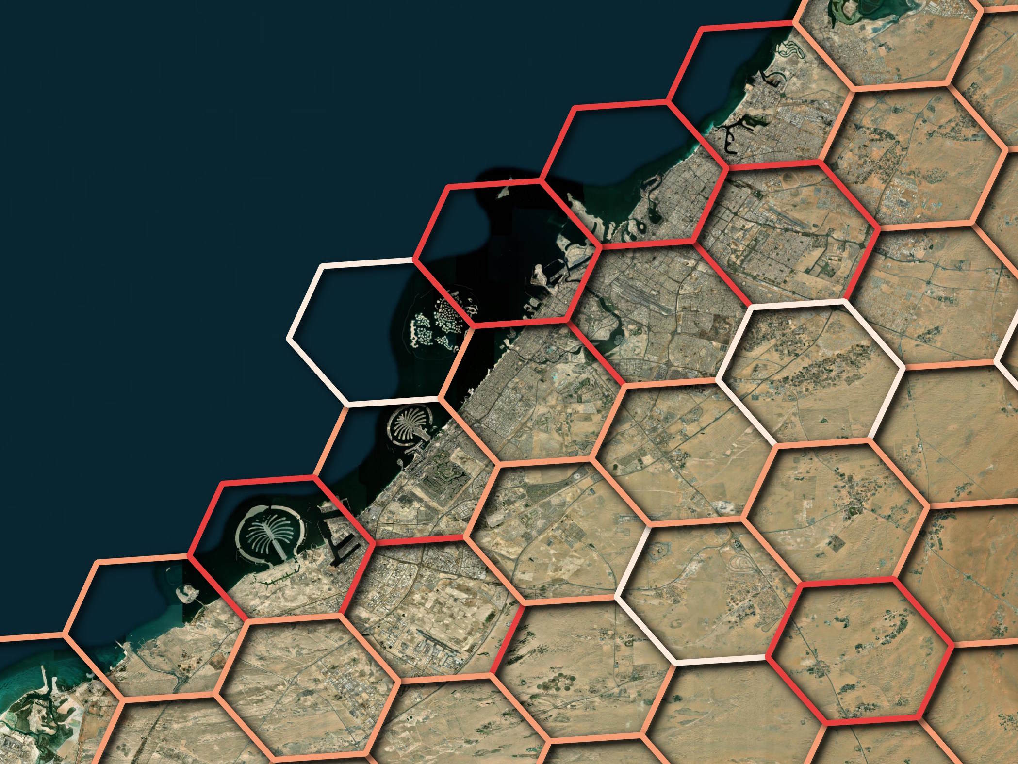
For reference, you'd only need a dozen or so of these hexagons to cover Dubai's urban areas.
Buildings in Beijing
Last year, I wrote a blog post about a team of researchers that built an AI-detected building dataset from Google Map's Satellite Imagery. The dataset uses the acronym CLSM. It did a lot to fill in the many missing areas of China that aren't mapped on OpenStreetMap (OSM). This dataset ended up being the bulk of Overture's building dataset for China earlier this year.
In some areas, CLSM did a great job of accurately identifying building footprints but there were other areas where the model wasn't as accurate.
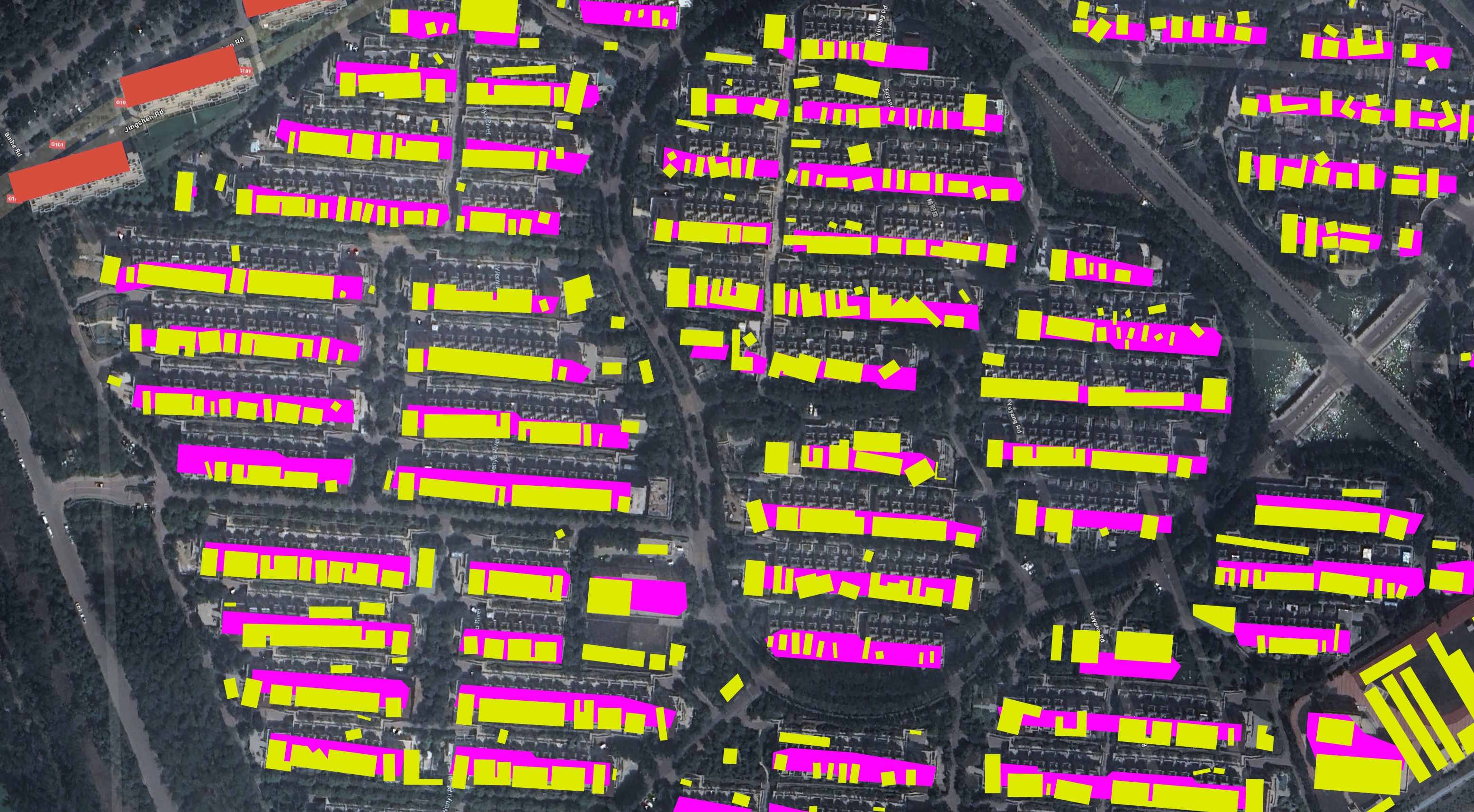
Below in yellow is CLSM's data for a neighbourhood in Beijing. In purple is GBA's. As you can see, there has been a serious improvement in accuracy.
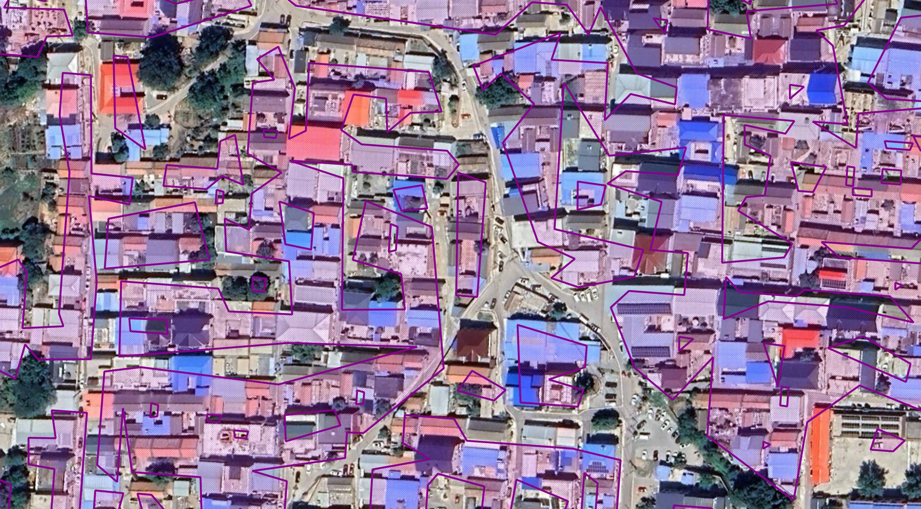
Still, GBA isn't without its faults. This is another neighbourhood in Beijing.
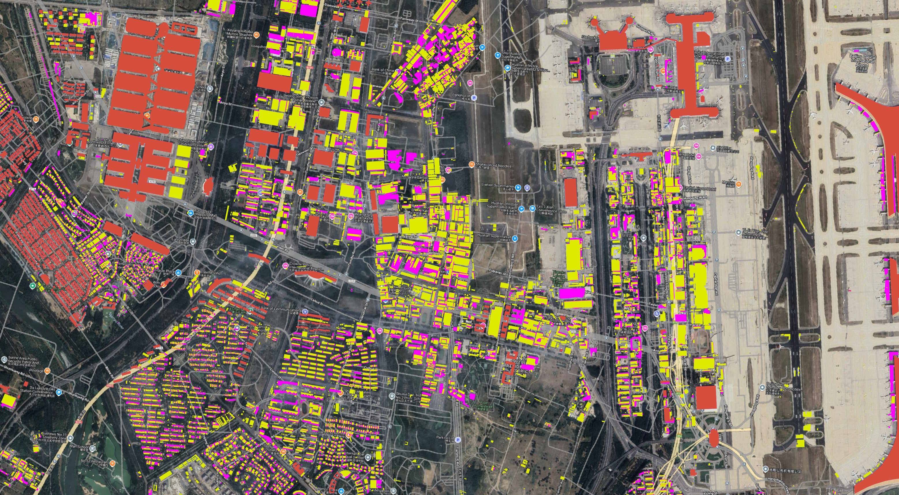
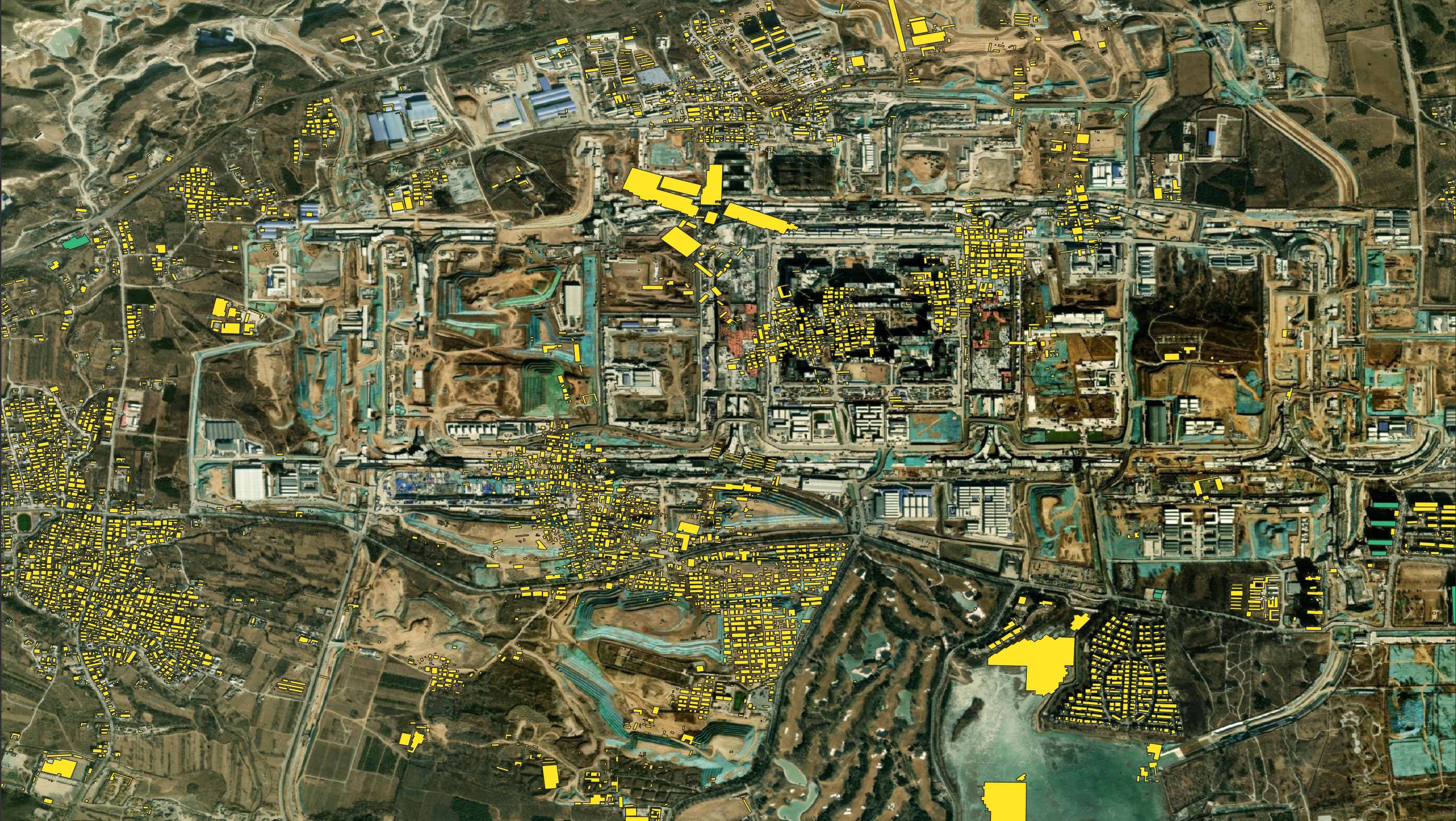
Below is the area around Beijing's Capital International Airport (PEK). Red is OSM, yellow is CLSM (via Overture) and purple is the AI-generated GBA building footprints that I believe were built exclusively from deep learning on Planet Labs' imagery.
Ultimately, map makers are left needing to do a pick-and-mix approach to cleaning up this data. That said, where GBA can't be the final deliverable, it can at least help speed up the process.
Lack of Timestamps
China is currently building the world's largest military command centre. It's located at 116.06753 East, 39.81821 North.
As of this writing, the satellite map images from Bing and Yandex show the village that used to be here a few years ago before construction began. Below is a rendering of GBA's building footprints for this area on top of a satellite image from Yandex.
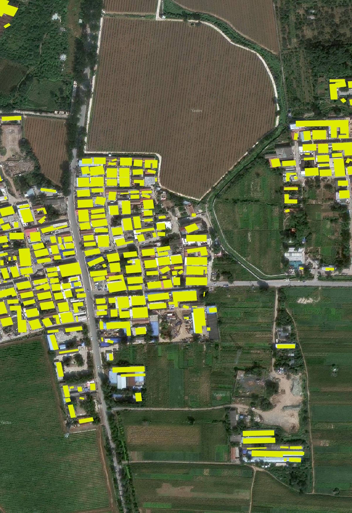
The buildings shown aren't from GBA's "ours2" dataset but rather old OSM data. This is what OSM currently looks like.
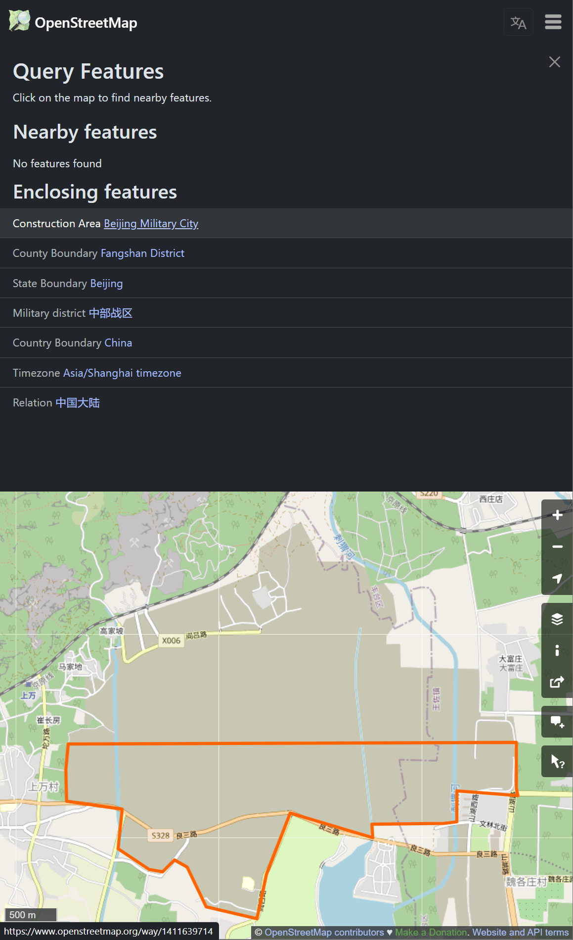
Esri has a relatively recent image of this area. Below you can see GBA's data on top of it.
As GBA has now been published and there hasn't been any announcement of upcoming updates, any priority on conflicting footprints should go in favour of the latest OSM building footprints.
For specific areas with a lot of construction, it might be worth excluding any OSM-sourced buildings in GBA's dataset entirely and use Overture's latest feed instead. Overture prioritise OSM data that will be, at most, weeks old when available.
Planet Labs' Metadata
The timestamp issue is more than just old OSM data. Any of GBA's AI-generated building footprints fails to identify the date of capture of the imagery they ran inference on. It would have been great if they had included Planet Labs' metadata in each of their records.
Countries
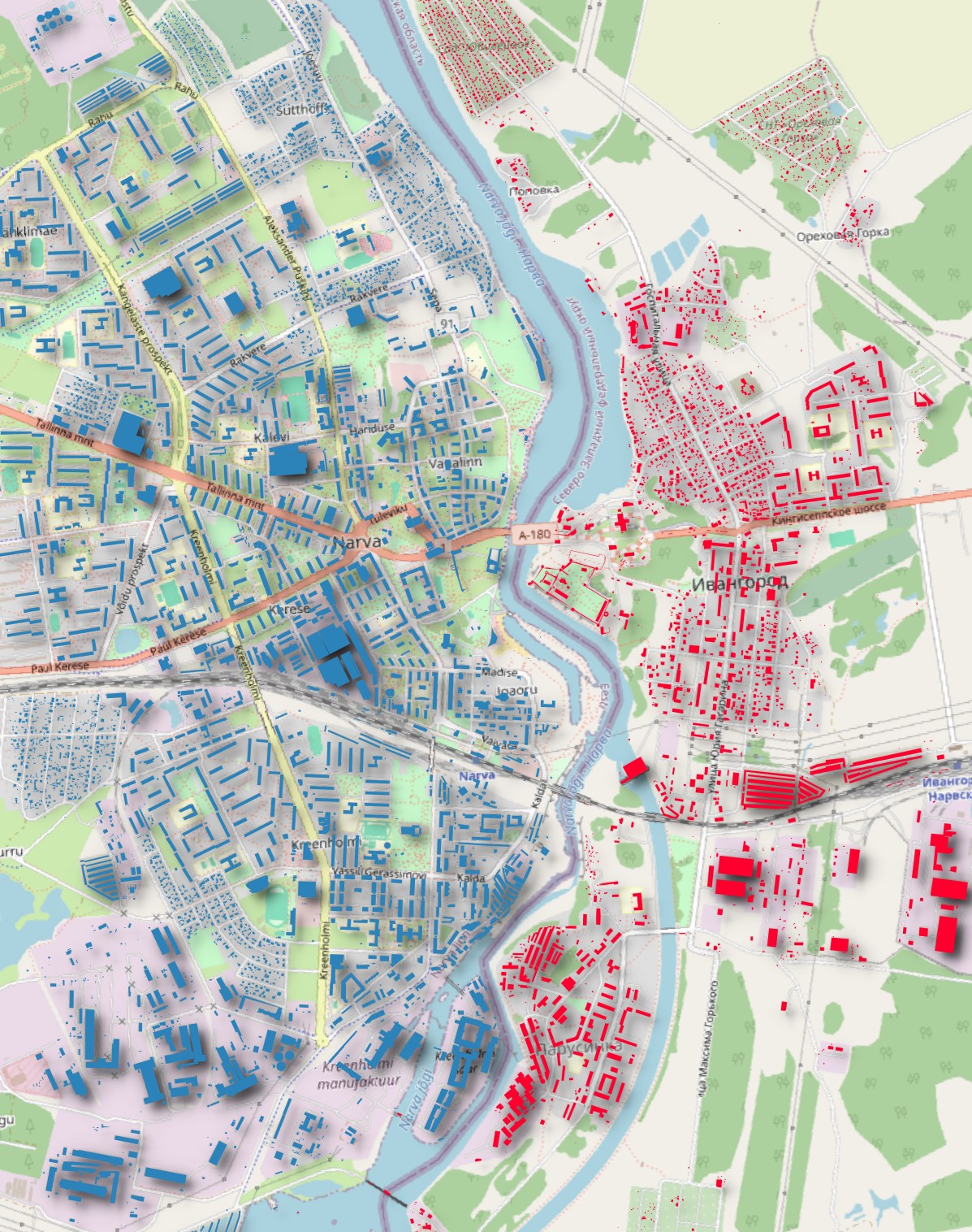
Border towns can often get marked as being in another country in datasets I come across. I'm pleased to say I haven't found this issue in this dataset.
Below is Narva, Estonia's buildings in blue and Ivangorod, Russia's in red. All of the buildings appear to be correctly marked with the country they're located in.
Below are the building counts, rounded to the nearest million for the top 40 most prominent countries in this dataset.
$ ~/duckdb
SELECT   ROUND(COUNT(*) / 1_000_000)::INT AS num_buildings,
         region
FROM     READ_PARQUET('*.parquet')
GROUP BY 2
ORDER BY 1 DESC
LIMIT    40;
┌───────────────┬─────────┐
│ num_buildings │ region  │
│     int32     │ varchar │
├───────────────┼─────────┤
│           467 │ IND     │
│           165 │ CHN     │
│           151 │ USA     │
│           139 │ BRA     │
│           115 │ IDN     │
│            84 │ MEX     │
│            74 │ RUS     │
│            67 │ NGA     │
│            62 │ PAK     │
│            60 │ VNM     │
│            53 │ FRA     │
│            51 │ JPN     │
│            48 │ THA     │
│            43 │ DEU     │
│            43 │ ZAF     │
│            40 │ BGD     │
│            38 │ ETH     │
│            35 │ PHL     │
│            33 │ ARG     │
│            30 │ TZA     │
│            28 │ KEN     │
│            28 │ UKR     │
│            27 │ SDN     │
│            26 │ COD     │
│            25 │ EGY     │
│            23 │ GBR     │
│            22 │ POL     │
│            22 │ UGA     │
│            21 │ TUR     │
│            21 │ ITA     │
│            21 │ PER     │
│            18 │ COL     │
│            18 │ MOZ     │
│            16 │ BFA     │
│            16 │ DZA     │
│            14 │ VEN     │
│            14 │ CHL     │
│            13 │ IRN     │
│            13 │ GHA     │
│            13 │ ROU     │
├───────────────┴─────────┤
│ 40 rows       2 columns │
└─────────────────────────┘
The 151M Buildings for the US is a bit of a surprise for me. The ORNL dataset for last year had this number at 131M which included building usage and addresses.
The Height Dataset
35 of the 36 TB of data TUM published is made up of GeoTIFF height maps stored in ZIP files. Each ZIP file contains 100s of GeoTIFFs.
$ wget -c "https://dataserv.ub.tum.de/public.php/dav/files/m1782307/Height/africa/e000_n10_e005_n05.zip"
The above 96 GB ZIP file contains a total of 114.5 GB worth of GeoTIFFs.
$ unzip -l e000_n10_e005_n05.zip
Archive:  e000_n10_e005_n05.zip
  Length      Date    Time    Name
---------  ---------- -----   ----
266161026  2024-04-19 18:16   0.0_9.2_0.2_9.0_sr_ss.tif
264664332  2024-04-19 22:05   1.2_7.4_1.4_7.2_sr_ss.tif
...
262812174  2024-04-20 04:38   3.6_8.4_3.8_8.2_sr_ss.tif
264402340  2024-04-20 07:33   4.8_9.0_5.0_8.8_sr_ss.tif
---------                     -------
114525128728                     434 files
Below is one of the height maps rendered in QGIS.
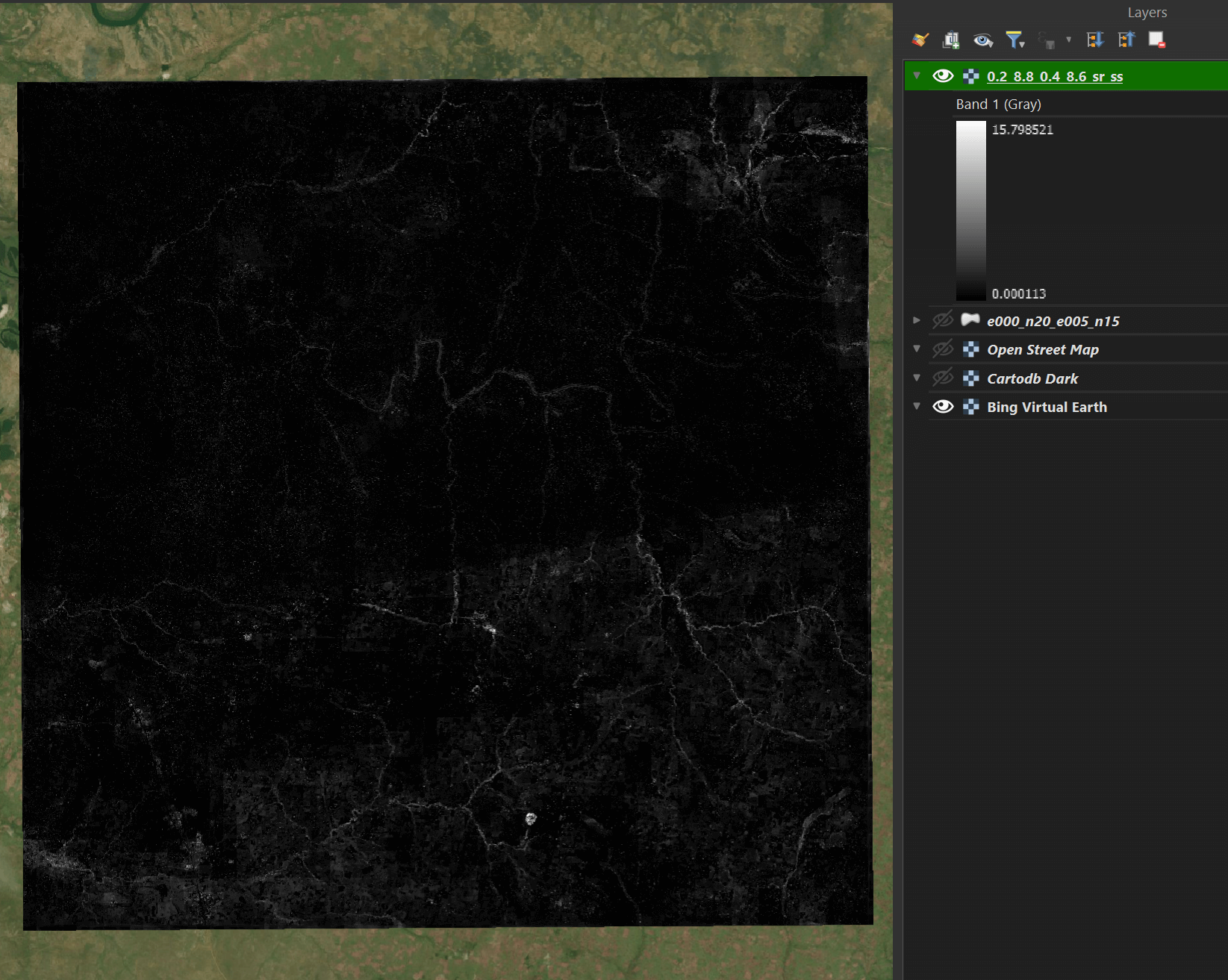
Below is the metadata on the above 254 MB GeoTIFF.
$ exiftool 0.2_8.8_0.4_8.6_sr_ss.tif \
    | jc --kv \
    | jq -S .
{
  "Bits Per Sample": "32",
  "Compression": "Uncompressed",
  "Directory": ".",
  "Exif Byte Order": "Little-endian (Intel, II)",
  "ExifTool Version Number": "12.76",
  "File Access Date/Time": "2025:09:02 19:17:14+03:00",
  "File Inode Change Date/Time": "2025:09:02 18:16:24+03:00",
  "File Modification Date/Time": "2024:04:19 18:52:54+03:00",
  "File Name": "0.2_8.8_0.4_8.6_sr_ss.tif",
  "File Permissions": "-rwxrwxrwx",
  "File Size": "266 MB",
  "File Type": "TIFF",
  "File Type Extension": "tif",
  "GDAL No Data": "-1",
  "GT Citation": "WGS 84 / UTM zone 31N",
  "GT Model Type": "Projected",
  "GT Raster Type": "Pixel Is Area",
  "Geo Tiff Version": "1.1.0",
  "Geog Angular Units": "Angular Degree",
  "Geog Citation": "WGS 84",
  "Image Height": "8172",
  "Image Size": "8133x8172",
  "Image Width": "8133",
  "MIME Type": "image/tiff",
  "Megapixels": "66.5",
  "Model Tie Point": "0 0 0 190683 975006 0",
  "Photometric Interpretation": "BlackIsZero",
  "Pixel Scale": "3 3 0",
  "Planar Configuration": "Chunky",
  "Proj Linear Units": "Linear Meter",
  "Projected CS Type": "WGS84 UTM zone 31N",
  "Rows Per Strip": "1",
  "Sample Format": "Float",
  "Samples Per Pixel": "1",
  "Strip Byte Counts": "(Binary data 49031 bytes, use -b option to extract)",
  "Strip Offsets": "(Binary data 78308 bytes, use -b option to extract)"
}