On September 12th, Public Safety Canada (PSC) released Canada Structures. This dataset contains 13,760,754 Canadian building footprints; many with heights and metadata describing their usage.
They sourced data from OpenStreetMap (OSM), Microsoft Building Footprints (MSB), Open Data Base of Buildings (ODB) and height data was collected from Natural Resources Canada.
The dataset was assembled in April 2024. The ODB data, which is a collection of data from municipalities of Canada, was from 2019, not the newer 2025 release.
I'm not certain when they collected their data from OSM but I found records from February 2023 that didn't make the cut into this release.
The MSB data was likely version 1.1 which was published in June of 2019.
Below is a heatmap of the building footprints.
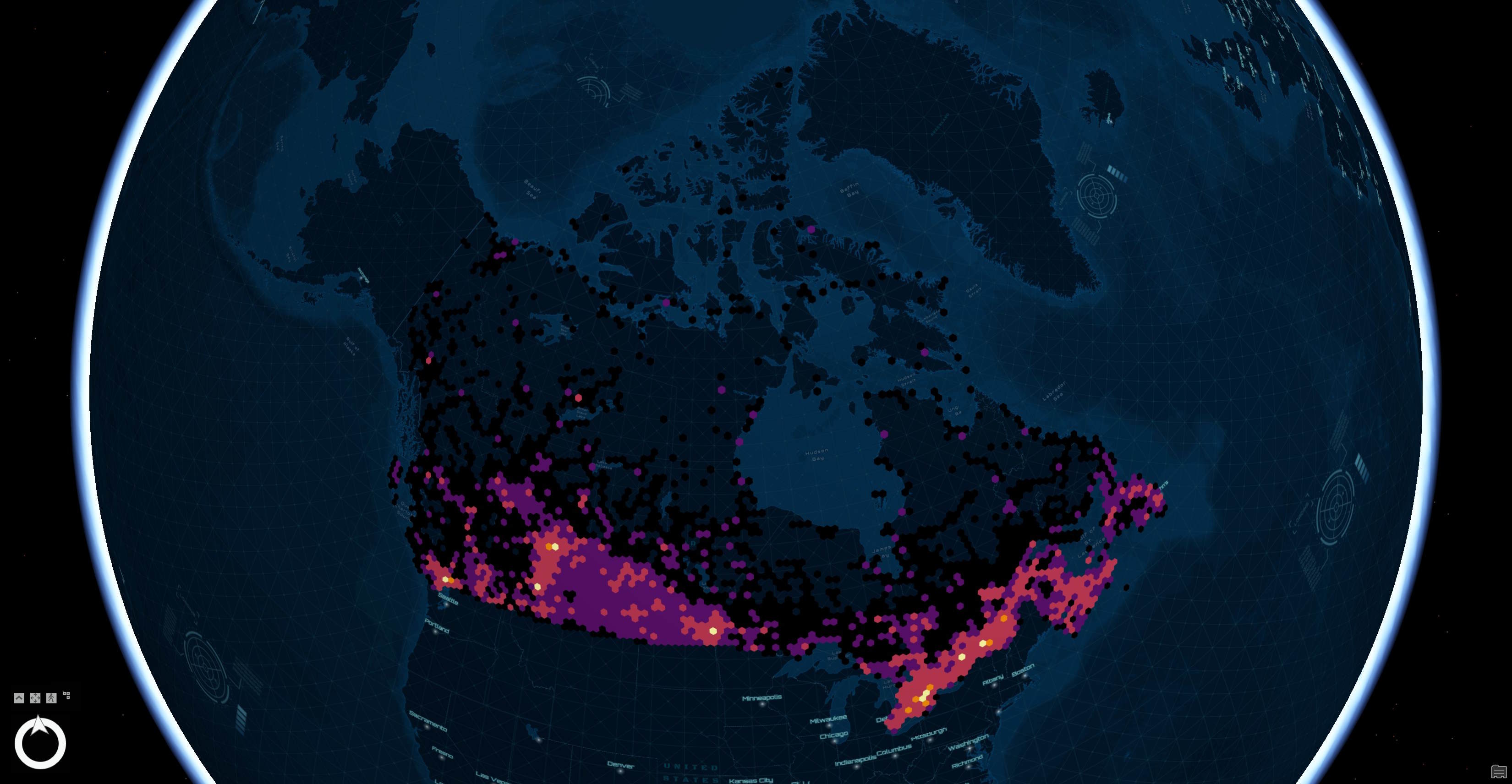
In this post, I'll explore Canada Structures' version 1.0.0.
My Workstation
I'm using a 5.7 GHz AMD Ryzen 9 9950X CPU. It has 16 cores and 32 threads and 1.2 MB of L1, 16 MB of L2 and 64 MB of L3 cache. It has a liquid cooler attached and is housed in a spacious, full-sized Cooler Master HAF 700 computer case.
The system has 96 GB of DDR5 RAM clocked at 4,800 MT/s and a 5th-generation, Crucial T700 4 TB NVMe M.2 SSD which can read at speeds up to 12,400 MB/s. There is a heatsink on the SSD to help keep its temperature down. This is my system's C drive.
The system is powered by a 1,200-watt, fully modular Corsair Power Supply and is sat on an ASRock X870E Nova 90 Motherboard.
I'm running Ubuntu 24 LTS via Microsoft's Ubuntu for Windows on Windows 11 Pro. In case you're wondering why I don't run a Linux-based desktop as my primary work environment, I'm still using an Nvidia GTX 1080 GPU which has better driver support on Windows and ArcGIS Pro only supports Windows natively.
Installing Prerequisites
I'll use GDAL 3.9.3 and a few other tools to help analyse the data in this post.
$ sudo add-apt-repository ppa:ubuntugis/ubuntugis-unstable
$ sudo apt update
$ sudo apt install \
    gdal-bin \
    jq
I'll use DuckDB, along with its H3, JSON, Lindel, Parquet and Spatial extensions, in this post.
$ cd ~
$ wget -c https://github.com/duckdb/duckdb/releases/download/v1.3.2/duckdb_cli-linux-amd64.zip
$ unzip -j duckdb_cli-linux-amd64.zip
$ chmod +x duckdb
$ ~/duckdb
INSTALL h3 FROM community;
INSTALL lindel FROM community;
INSTALL json;
INSTALL parquet;
INSTALL spatial;
I'll set up DuckDB to load every installed extension each time it launches.
$ vi ~/.duckdbrc
.timer on
.width 180
LOAD h3;
LOAD lindel;
LOAD json;
LOAD parquet;
LOAD spatial;
The maps in this post were mostly rendered with QGIS version 3.44. QGIS is a desktop application that runs on Windows, macOS and Linux. The application has grown in popularity in recent years and has ~15M application launches from users all around the world each month.
I used QGIS' Tile+ plugin to add basemaps from Google and OpenStreetMap (OSM) to the maps throughout this post.
Analysis-Ready Data
PSC broke up the dataset into GeoPackage (GPKG) files by province / territory. Below I'll build a manifest of these URLs and download them with four concurrent threads.
$ mkdir -p ~/psc
$ cd ~/psc

$ vi urls.txt
https://open.canada.ca/data/dataset/3829eee9-f898-4643-9ad8-f48575b8873d/resource/909a44d6-1040-408d-896e-7362d2165688/download/ab_structures_en.gpkg
https://open.canada.ca/data/dataset/3829eee9-f898-4643-9ad8-f48575b8873d/resource/d858fd57-2c9a-4978-bc50-79aef286bccf/download/mb_structures_en.gpkg
https://open.canada.ca/data/dataset/3829eee9-f898-4643-9ad8-f48575b8873d/resource/f7fdee7d-09dd-4eb6-88fd-2234ad701309/download/on_structures_en.gpkg
https://open.canada.ca/data/dataset/3829eee9-f898-4643-9ad8-f48575b8873d/resource/71db1a0f-0099-4fbe-ad9a-f51626506e8a/download/qc_structures_en.gpkg
https://open.canada.ca/data/dataset/3829eee9-f898-4643-9ad8-f48575b8873d/resource/5490a8a0-753a-41f7-8ab5-d3870ee0ea69/download/bc_structures_en.gpkg
https://open.canada.ca/data/dataset/3829eee9-f898-4643-9ad8-f48575b8873d/resource/b903c565-8fdc-453e-9927-8b1a33829d07/download/ns_structures_en.gpkg
https://open.canada.ca/data/dataset/3829eee9-f898-4643-9ad8-f48575b8873d/resource/f4a95ecb-5b58-4021-a591-ca1d8b2bbae4/download/sk_structures_en.gpkg
https://open.canada.ca/data/dataset/3829eee9-f898-4643-9ad8-f48575b8873d/resource/610fb5b5-e12c-41a1-aa28-415b51c24333/download/nt_structures_en.gpkg
https://open.canada.ca/data/dataset/3829eee9-f898-4643-9ad8-f48575b8873d/resource/d892ce68-bcd8-463b-a2fa-0439ef75c2b8/download/pe_structures_en.gpkg
https://open.canada.ca/data/dataset/3829eee9-f898-4643-9ad8-f48575b8873d/resource/680f47b9-9e23-4888-9950-10e561ae0556/download/nl_structures_en.gpkg
https://open.canada.ca/data/dataset/3829eee9-f898-4643-9ad8-f48575b8873d/resource/fcd7fe5b-be3e-4499-8b6e-11ce5ca391cc/download/nu_structures_en.gpkg
https://open.canada.ca/data/dataset/3829eee9-f898-4643-9ad8-f48575b8873d/resource/15737be6-24f3-4764-b40c-6f23f8dd44e0/download/yk_structures_en.gpkg
https://open.canada.ca/data/dataset/3829eee9-f898-4643-9ad8-f48575b8873d/resource/6ff6252a-50f4-43b6-b6d0-7d6d904a3e68/download/nb_structures_en.gpkg
$ cat urls.txt \
    | xargs -n1 \
            -P4 \
            -I% \
            wget -c "%"
I'll extract the projection PSC used. This proj4 string will be used to below to re-project the data into EPSG:4326.
$ gdalsrsinfo \
    -o proj4 \
    ab_structures_en.gpkg
+proj=lcc +lat_0=63.390675 +lon_0=-91.8666666666667 +lat_1=49 +lat_2=77 +x_0=6200000 +y_0=3000000 +ellps=GRS80 +units=m +no_defs
I'll convert the GPKG files into spatially-sorted, ZStandard-compressed Parquet format with an EPSG:4326 projection. I've also made a clear source field and added bounding boxes to each piece of geometry.
This format will load without issue in QGIS 3.44 and ArcGIS Pro 3.5. The bounding boxes will help optimise bandwidth usage when querying this data on remote servers, like AWS S3.
$ for FILENAME in *.gpkg; do
     echo $FILENAME

     BASENAME=`basename $FILENAME | cut -d. -f1`

     echo "COPY (
               WITH a AS (
                   SELECT * EXCLUDE(geom),
                          ST_FLIPCOORDINATES(
                              ST_TRANSFORM(
                                  geom,
                                  '+proj=lcc +lat_0=63.390675  +lon_0=-91.8666666666667 +lat_1=49  +lat_2=77 +x_0=6200000 +y_0=3000000  +ellps=GRS80 +units=m +no_defs  +type=crs',
                                  'EPSG:4326')) geometry
                   FROM ST_READ('$FILENAME')
               )
               SELECT   *,
                        {'xmin': ST_XMIN(ST_EXTENT(geometry)),
                         'ymin': ST_YMIN(ST_EXTENT(geometry)),
                         'xmax': ST_XMAX(ST_EXTENT(geometry)),
                         'ymax': ST_YMAX(ST_EXTENT(geometry))} AS bbox,
                         CASE WHEN MSB IS NOT NULL THEN 'MSB'
                              WHEN ODB IS NOT NULL THEN 'ODB'
                              WHEN OSM IS NOT NULL THEN 'OSM'
                         END AS source
               FROM     a
               ORDER BY HILBERT_ENCODE([ST_Y(ST_CENTROID(geometry)),
                                        ST_X(ST_CENTROID(geometry))]::double[2])
           ) TO '$BASENAME.parquet' (
               FORMAT            'PARQUET',
               CODEC             'ZSTD',
               COMPRESSION_LEVEL 22,
               ROW_GROUP_SIZE    15000);
           " | ~/duckdb
 done
The above turned 3.9 GB of GPKG files into 1.5 GB of Parquet.
$ du -hsc *structures_en.parquet
197M    ab_structures_en.parquet
169M    bc_structures_en.parquet
69M     mb_structures_en.parquet
40M     nb_structures_en.parquet
26M     nl_structures_en.parquet
51M     ns_structures_en.parquet
2.9M    nt_structures_en.parquet
1.1M    nu_structures_en.parquet
536M    on_structures_en.parquet
7.6M    pe_structures_en.parquet
276M    qc_structures_en.parquet
71M     sk_structures_en.parquet
1.6M    yk_structures_en.parquet
1.5G    total
Heatmap
Below is a heatmap of this dataset.
CREATE OR REPLACE TABLE h3_4_stats AS
    SELECT   H3_LATLNG_TO_CELL(
                bbox.ymin,
                bbox.xmin, 4) AS h3_4,
             COUNT(*) num_buildings
    FROM     READ_PARQUET('*_structures_en.parquet')
    WHERE    bbox.xmin BETWEEN -178.5 AND 178.5
    GROUP BY 1;

COPY (
    SELECT ST_ASWKB(H3_CELL_TO_BOUNDARY_WKT(h3_4)::geometry) geometry,
           num_buildings
    FROM   h3_4_stats
) TO 'h3_4_stats.gpkg'
  WITH (FORMAT GDAL,
        DRIVER 'GPKG',
        LAYER_CREATION_OPTIONS 'WRITE_BBOX=YES');
The following was needed for ArcGIS Pro to recognise the projection of the above hexagons properly.
$ ogr2ogr \
    -f GPKG \
    -a_srs EPSG:4326 \
    h3_4_stats.4326.gpkg \
    h3_4_stats.gpkg
Data Fluency
Below are the field names, data types, percentages of NULLs per column, number of unique values and minimum and maximum values for each column.
$ ~/duckdb
SELECT   column_name,
         column_type,
         null_percentage,
         approx_unique,
         min,
         max
FROM     (SUMMARIZE
          FROM READ_PARQUET('*_structures_en.parquet'))
WHERE    column_name != 'geometry'
AND      column_name != 'bbox'
ORDER BY 1;
┌─────────────┬─────────────┬─────────────────┬───────────────┬───────────────────┬────────────────────┐
│ column_name │ column_type │ null_percentage │ approx_unique │        min        │        max         │
│   varchar   │   varchar   │  decimal(9,2)   │     int64     │      varchar      │      varchar       │
├─────────────┼─────────────┼─────────────────┼───────────────┼───────────────────┼────────────────────┤
│ Area        │ DOUBLE      │            0.00 │      14644202 │ 0.00022589575436  │ 2788966.1142695914 │
│ CS_ID       │ BIGINT      │            0.00 │      12278694 │ 1                 │ 13763995           │
│ Height      │ DOUBLE      │           13.72 │       8158934 │ 0.0               │ 270.43516061452516 │
│ LC_Name     │ VARCHAR     │           96.04 │         19469 │ "Sifton Cemetery" │ Ïles aux Chats     │
│ MSB         │ VARCHAR     │           50.69 │             1 │ 1                 │ 1                  │
│ ODB         │ VARCHAR     │           67.74 │             1 │ 1                 │ 1                  │
│ ODB_ID      │ VARCHAR     │           67.74 │       4186001 │ 12010010000001    │ 61060970000014     │
│ ODB_Source  │ VARCHAR     │           67.74 │            66 │ Airdrie           │ York Region        │
│ OSM         │ VARCHAR     │           56.89 │             1 │ 1                 │ 1                  │
│ OSM_ID      │ VARCHAR     │           56.89 │       6684280 │ 1000016583        │ j                  │
│ OSM_LC      │ VARCHAR     │           32.15 │            16 │ allotments        │ vineyard           │
│ OSM_Name    │ VARCHAR     │           99.10 │         95599 │ "8-Building"      │ étable             │
│ OSM_Type    │ VARCHAR     │           82.44 │           358 │ Administratif     │ yurt               │
│ Perimeter   │ DOUBLE      │            0.00 │      13164420 │ 0.107992344195257 │ 16624.67147343245  │
│ Province    │ VARCHAR     │            0.00 │            12 │ AB                │ YK                 │
│ source      │ VARCHAR     │            0.00 │             3 │ MSB               │ OSM                │
├─────────────┴─────────────┴─────────────────┴───────────────┴───────────────────┴────────────────────┤
│ 16 rows                                                                                    6 columns │
└──────────────────────────────────────────────────────────────────────────────────────────────────────┘
Sources
This is the breakdown of records per source per province. There is a clear preference for MSB with ODB often completely absent.
$ ~/duckdb
WITH a AS (
    SELECT   Province,
             source,
             COUNT(*) cnt
    FROM     '*_structures_en.parquet'
    GROUP BY 1, 2)
PIVOT    a
ON       source
USING    SUM(cnt)
GROUP BY Province
ORDER BY 2 DESC;
┌──────────┬─────────┬─────────┬────────┐
│ Province │   MSB   │   ODB   │  OSM   │
│ varchar  │ int128  │ int128  │ int128 │
├──────────┼─────────┼─────────┼────────┤
│ QC       │ 1798578 │  491156 │ 504603 │
│ ON       │ 1333101 │ 2465651 │ 934046 │
│ AB       │ 1082368 │  495617 │ 332508 │
│ BC       │  688603 │  556590 │ 290223 │
│ MB       │  638831 │    NULL │  82979 │
│ SK       │  509567 │   98226 │ 130160 │
│ NL       │  255350 │    NULL │  32917 │
│ NB       │  216369 │   95832 │  91412 │
│ NS       │  168198 │  230801 │ 108674 │
│ PE       │   77119 │    NULL │   4567 │
│ YK       │   11563 │    NULL │   4461 │
│ NT       │    3192 │    5835 │  10589 │
│ NU       │    2882 │    NULL │   8186 │
├──────────┴─────────┴─────────┴────────┤
│ 13 rows                     4 columns │
└───────────────────────────────────────┘
The following is an example record which has been attributed to OSM.
$ echo "FROM  'ab_structures_en.parquet'
        WHERE source = 'OSM'
        LIMIT 1" \
    | ~/duckdb -json \
    | jq -S .
[
  {
    "Area": 1951.60849850855,
    "CS_ID": 7889231,
    "Height": 0.0,
    "LC_Name": null,
    "MSB": null,
    "ODB": null,
    "ODB_ID": null,
    "ODB_Source": null,
    "OSM": "1",
    "OSM_ID": "385156020",
    "OSM_LC": "forest",
    "OSM_Name": null,
    "OSM_Type": "industrial",
    "Perimeter": 283.5263470280223,
    "Province": "AB",
    "bbox": "{'xmin': -110.42687370425128, 'ymin': 55.06546590051143, 'xmax': -110.4250928025303, 'ymax': 55.0657240008682}",
    "geometry": "POLYGON ((-110.42687370425128 55.06546590051143, -110.42687370423948 55.0657240008682, -110.4250928025303 55.065687100742686, -110.42509280279089 55.06555190107596, -110.42655190404591 55.06558880094082, -110.42655190337649 55.06546590070232, -110.42687370425128 55.06546590051143))",
    "source": "OSM"
  }
]
As the following shows, records which are not attributed to OSM can still contain OSM metadata.
$ echo "FROM  'ab_structures_en.parquet'
        WHERE source = 'MSB'
        LIMIT 1" \
    | ~/duckdb -json \
    | jq -S .
[
  {
    "Area": 197.982910306995,
    "CS_ID": 8653450,
    "Height": 0.0,
    "LC_Name": "Cold Lake Air Weapons Range",
    "MSB": "1",
    "ODB": null,
    "ODB_ID": null,
    "ODB_Source": null,
    "OSM": null,
    "OSM_ID": null,
    "OSM_LC": "military",
    "OSM_Name": null,
    "OSM_Type": null,
    "Perimeter": 64.80059892006688,
    "Province": "AB",
    "bbox": "{'xmin': -110.59742700235742, 'ymin': 55.01551100079211, 'xmax': -110.59729400280793, 'ymax': 55.01572700092107}",
    "geometry": "POLYGON ((-110.59742700235742 55.01551100079211, -110.59742300421074 55.01572700092107, -110.59729400280793 55.015726000806524, -110.59729800362015 55.0155110012002, -110.59742700235742 55.01551100079211))",
    "source": "MSB"
  }
]
When ODB is used as a soruce, the ODB_Source column names the municipality the data came from. I'm a bit surprised to only see 64 unique values here.
.maxrows 20

SELECT   COUNT(*),
         ODB_Source
FROM     '*_structures_en.parquet'
WHERE    source  = 'ODB'
GROUP BY 2
ORDER BY 1 DESC;
┌──────────────┬─────────────────┐
│ count_star() │   ODB_Source    │
│    int64     │     varchar     │
├──────────────┼─────────────────┤
│       407142 │ Toronto         │
│       321334 │ Edmonton        │
│       320418 │ Ottawa          │
│       299972 │ York Region     │
│       253642 │ Durham          │
│       231396 │ Quebec          │
│       191918 │ Hamilton        │
│       144092 │ Halifax         │
│       133103 │ Surrey          │
│       130356 │ Brampton        │
│          ·   │    ·            │
│          ·   │    ·            │
│          ·   │    ·            │
│        10807 │ Cochrane        │
│         9027 │ New Westminster │
│         6839 │ Chestermere     │
│         6638 │ Squamish        │
│         5835 │ Yellowknife     │
│         5556 │ Canmore         │
│         5289 │ Whistler        │
│         5117 │ White Rock      │
│         1910 │ Banff           │
│          409 │ Sherbrooke      │
├──────────────┴─────────────────┤
│ 64 rows (20 shown)   2 columns │
└────────────────────────────────┘
Building Use
There are two fields, OSM_LC and OSM_Type, which can describe a building's use and surrounding area. Below are the record counts for the 21 unique values for OSM_LC. It's good to see most records are non-NULL.
SELECT   COUNT(*),
         OSM_LC
FROM     '*_structures_en.parquet'
GROUP BY 2
ORDER BY 1 DESC;
┌──────────────┬───────────────────┐
│ count_star() │      OSM_LC       │
│    int64     │      varchar      │
├──────────────┼───────────────────┤
│      7907072 │ residential       │
│      4423474 │ NULL              │
│       917211 │ forest            │
│       177327 │ industrial        │
│        94802 │ retail            │
│        79847 │ commercial        │
│        49464 │ farmyard          │
│        29279 │ park              │
│        27556 │ farmland          │
│        24495 │ nature_reserve    │
│         9042 │ military          │
│         4942 │ quarry            │
│         4847 │ grass             │
│         2934 │ cemetery          │
│         2921 │ recreation_ground │
│         2249 │ meadow            │
│         1787 │ scrub             │
│         1222 │ orchard           │
│          131 │ vineyard          │
│          108 │ allotments        │
│           44 │ heath             │
├──────────────┴───────────────────┤
│ 21 rows                2 columns │
└──────────────────────────────────┘
The OSM_Type has much more of a long tail and could probably do with some clustering. Also, out of the ~13M records in this dataset, this column is empty for 11.3M of them. There are also some values here, like industrial, which overlap with OSM_LC.
SELECT   COUNT(*),
         OSM_Type
FROM     '*_structures_en.parquet'
GROUP BY 2
ORDER BY 1 DESC;
┌──────────────┬──────────────────────┐
│ count_star() │       OSM_Type       │
│    int64     │       varchar        │
├──────────────┼──────────────────────┤
│     11344842 │ NULL                 │
│       864092 │ detached             │
│       766544 │ house                │
│       140230 │ residential          │
│       122762 │ garage               │
│       112894 │ terrace              │
│        67584 │ shed                 │
│        63904 │ apartments           │
│        41522 │ commercial           │
│        35143 │ industrial           │
│        32287 │ semidetached_house   │
│        30928 │ retail               │
│        25959 │ semi                 │
│        17495 │ farm_auxiliary       │
│        14288 │ static_caravan       │
│        14078 │ school               │
│         9024 │ roof                 │
│         8401 │ barn                 │
│         5980 │ cabin                │
│         5887 │ church               │
│            · │   ·                  │
│            · │   ·                  │
│            · │   ·                  │
│            1 │ residential;yes      │
│            1 │ air-supported        │
│            1 │ Control Tower        │
│            1 │ Banquet_Hall         │
│            1 │ hydro                │
│            1 │ outside              │
│            1 │ G                    │
│            1 │ changing_rooms       │
│            1 │ walkway              │
│            1 │ sse                  │
│            1 │ tourism              │
│            1 │ balcony              │
│            1 │ ramada_studio        │
│            1 │ military_armoury     │
│            1 │ Sports,_exercise_are │
│            1 │ Résidence_Maria-Gor  │
│            1 │ Hospital and Nursing │
│            1 │ recreational         │
│            1 │ social_facility      │
│            1 │ school;church        │
├──────────────┴──────────────────────┤
│ 401 rows (40 shown)       2 columns │
└─────────────────────────────────────┘
Below is the number of records with the above two fields populated broken down by source.
WITH a AS (
    SELECT   COUNT(*) cnt,
             source,
             OSM_LC   IS NOT NULL AS has_lc,
             OSM_Type IS NOT NULL AS has_type
    FROM     '*_structures_en.parquet'
    GROUP BY 2, 3, 4
)
PIVOT    a
ON       has_lc, has_type
USING    SUM(cnt)
GROUP BY source
ORDER BY 1;
┌─────────┬─────────────┬────────────┬────────────┬───────────┐
│ source  │ false_false │ false_true │ true_false │ true_true │
│ varchar │   int128    │   int128   │   int128   │  int128   │
├─────────┼─────────────┼────────────┼────────────┼───────────┤
│ MSB     │     3014756 │      22326 │    3676601 │     72038 │
│ ODB     │      552400 │     158812 │    2518475 │   1210021 │
│ OSM     │      490810 │     184370 │    1091800 │    768345 │
└─────────┴─────────────┴────────────┴────────────┴───────────┘
Building Heights
Not all buildings have heights. Below is the number of buildings that do broken down by source.
WITH a AS (
    SELECT   COUNT(*) cnt,
             source,
             Height > 0 AS has_height
    FROM     '*_structures_en.parquet'
    GROUP BY 2, 3
)
PIVOT    a
ON       has_height
USING    SUM(cnt)
GROUP BY source
ORDER BY 1;
┌─────────┬─────────┬─────────┐
│ source  │  false  │  true   │
│ varchar │ int128  │ int128  │
├─────────┼─────────┼─────────┤
│ MSB     │ 2078923 │ 3488475 │
│ ODB     │  145537 │ 4019747 │
│ OSM     │  491994 │ 1648099 │
└─────────┴─────────┴─────────┘
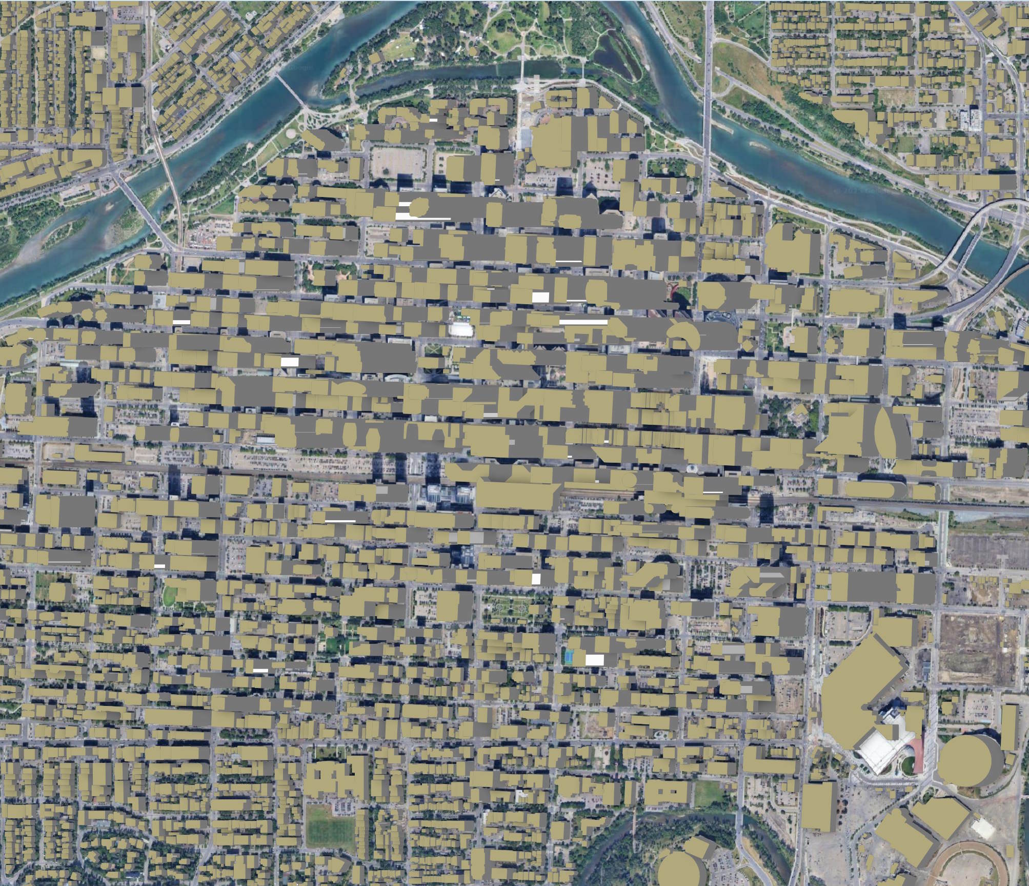
Building heights can look good at a distance. Below is Downtown Calgary.
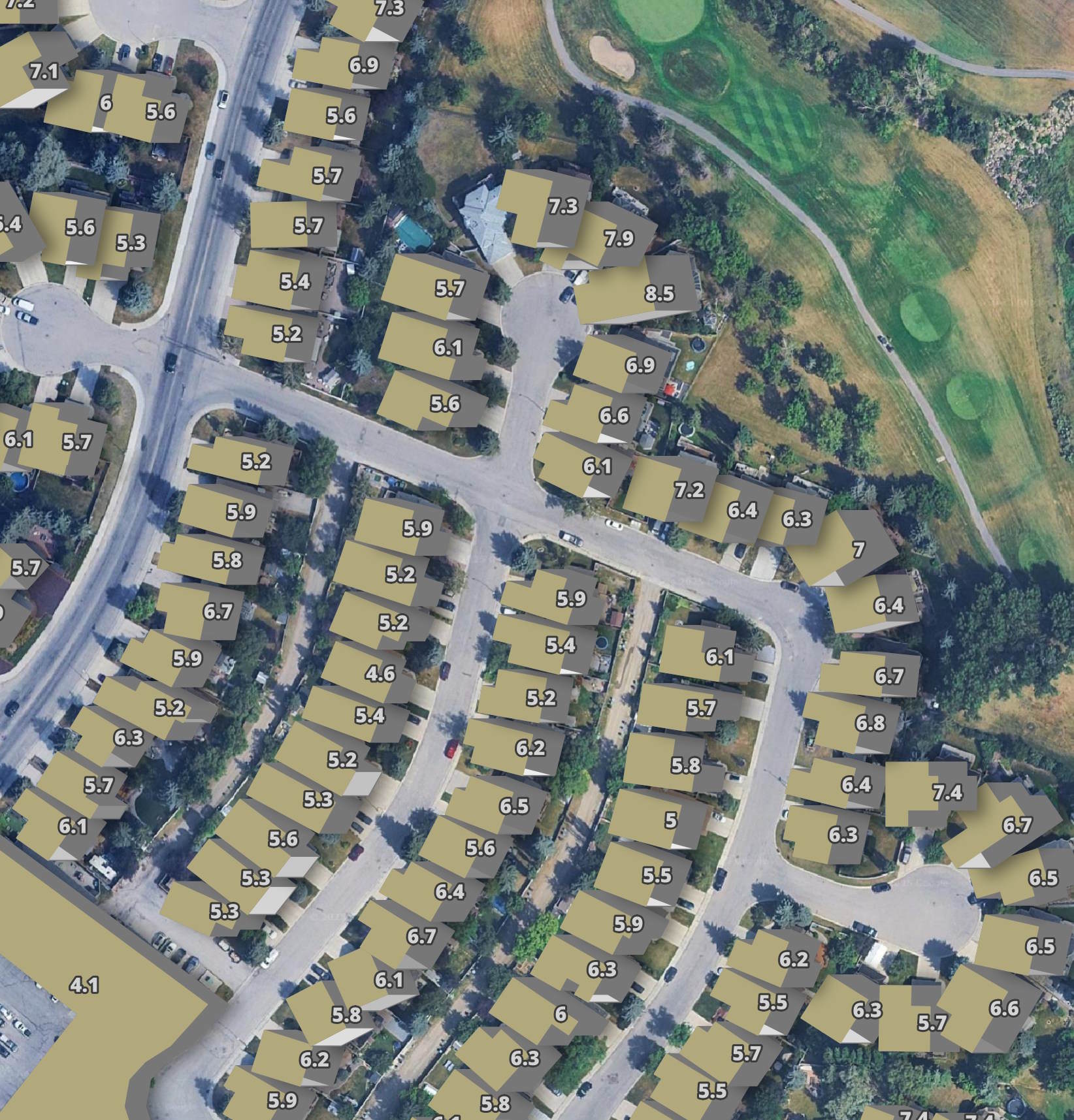
But in neighbourhoods with uniform housing, the heights can vary wildly. Below is Douglasdale in Calgary. The labels are each home's height, rounded to the nearest tenth.
Footprint Coverage
Buildings constructed after 2023 (or possibly even earlier) won't appear in this dataset. The image below is from South East Calgary. In yellow is the PSC's dataset with Overture's August release in purple.
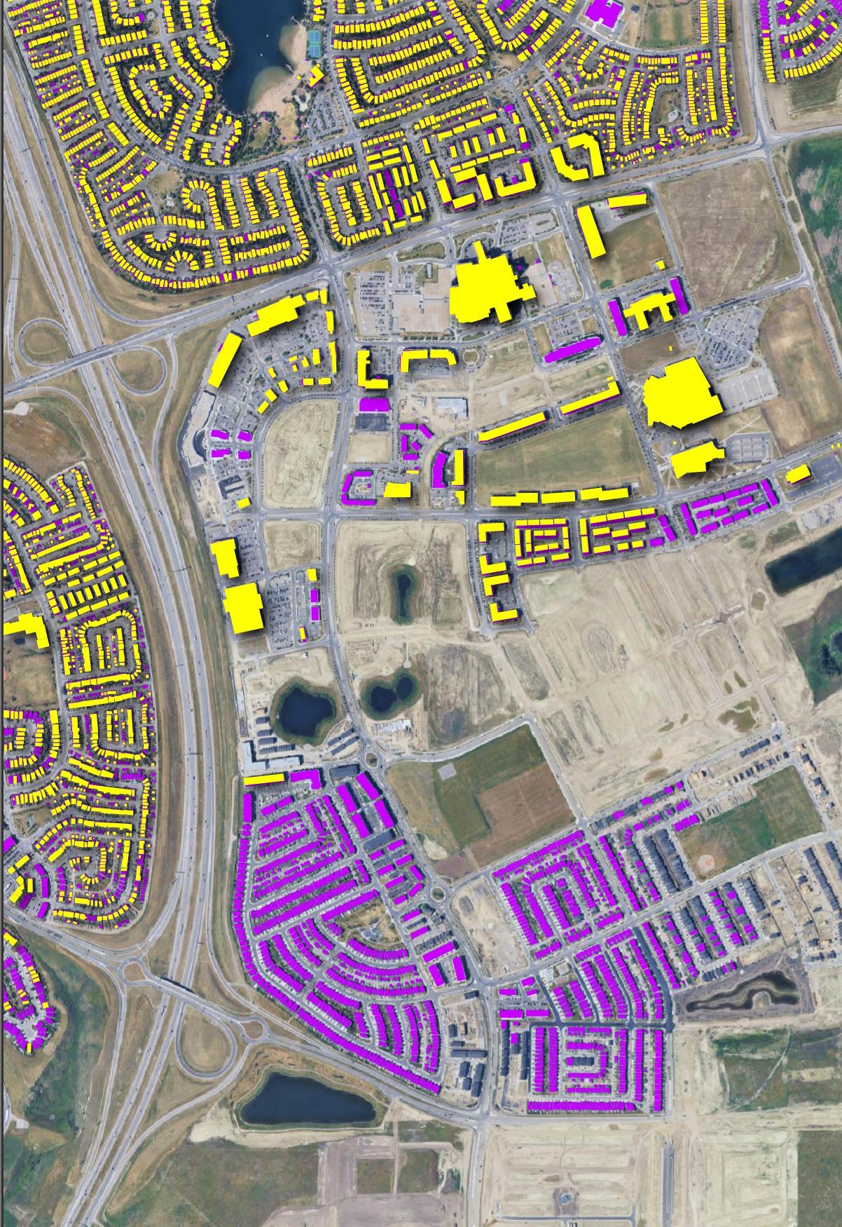
This is one of the purple areas on June 25th.
The TUM dataset I reviewed recently contains 305,208 fewer Canadian buildings than PSC's dataset. I couldn't find anywhere in Calgary where TUM data was the only footprint present.
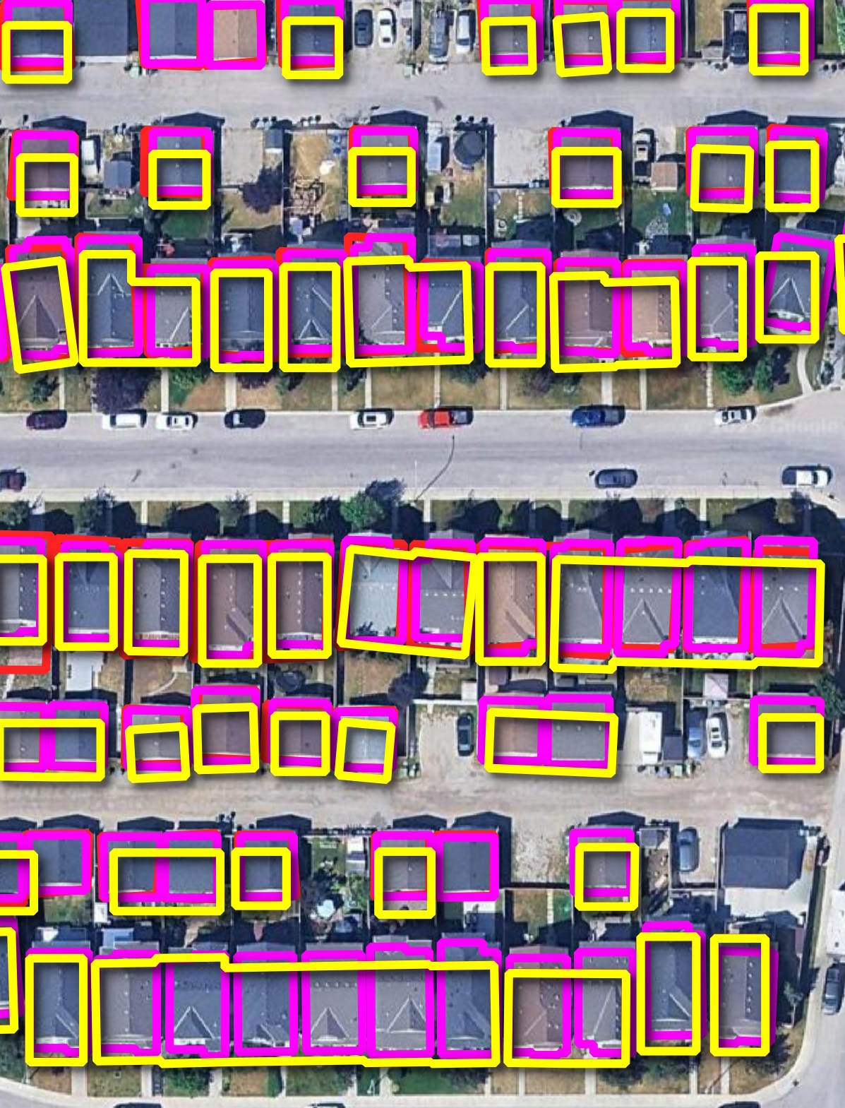
Some properties that are detached from one another are showing as being attached in this dataset. PSC's buildings are outlined in yellow, Overture in purple and TUM in red.
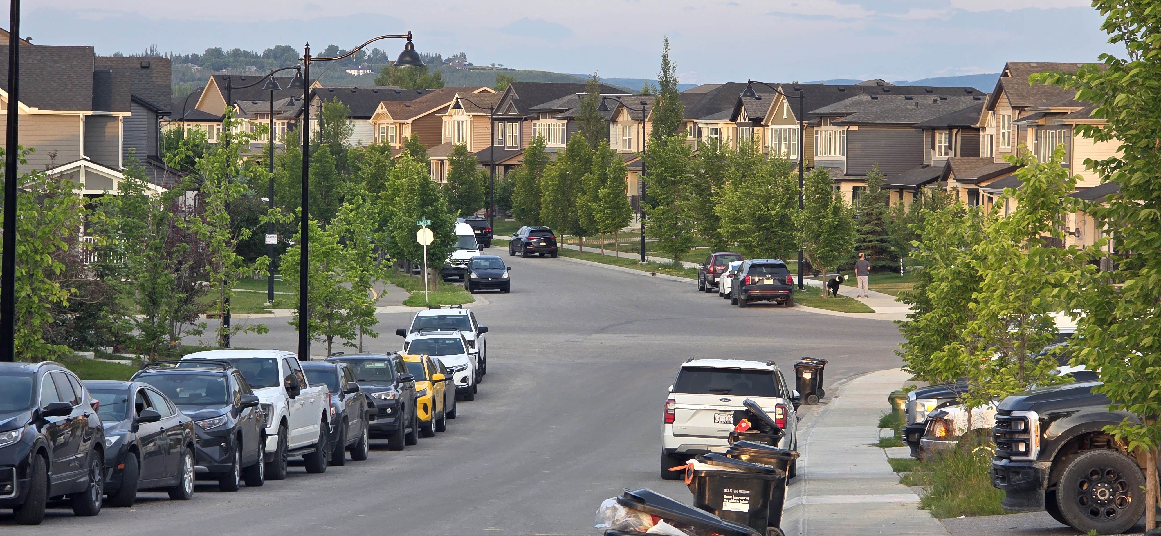
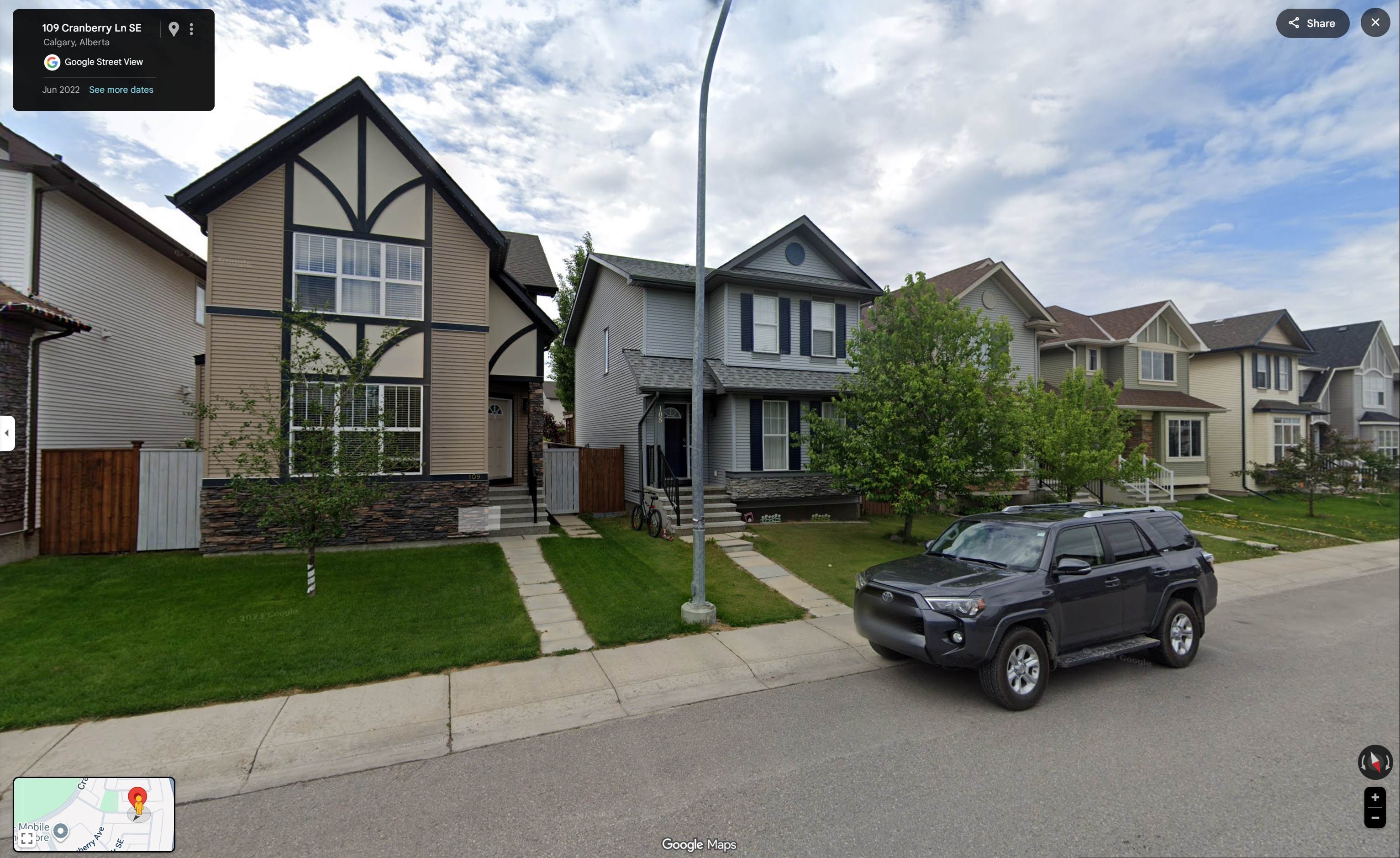
This is the same area on Google Streetview. As you can see, the houses are detached from one another.
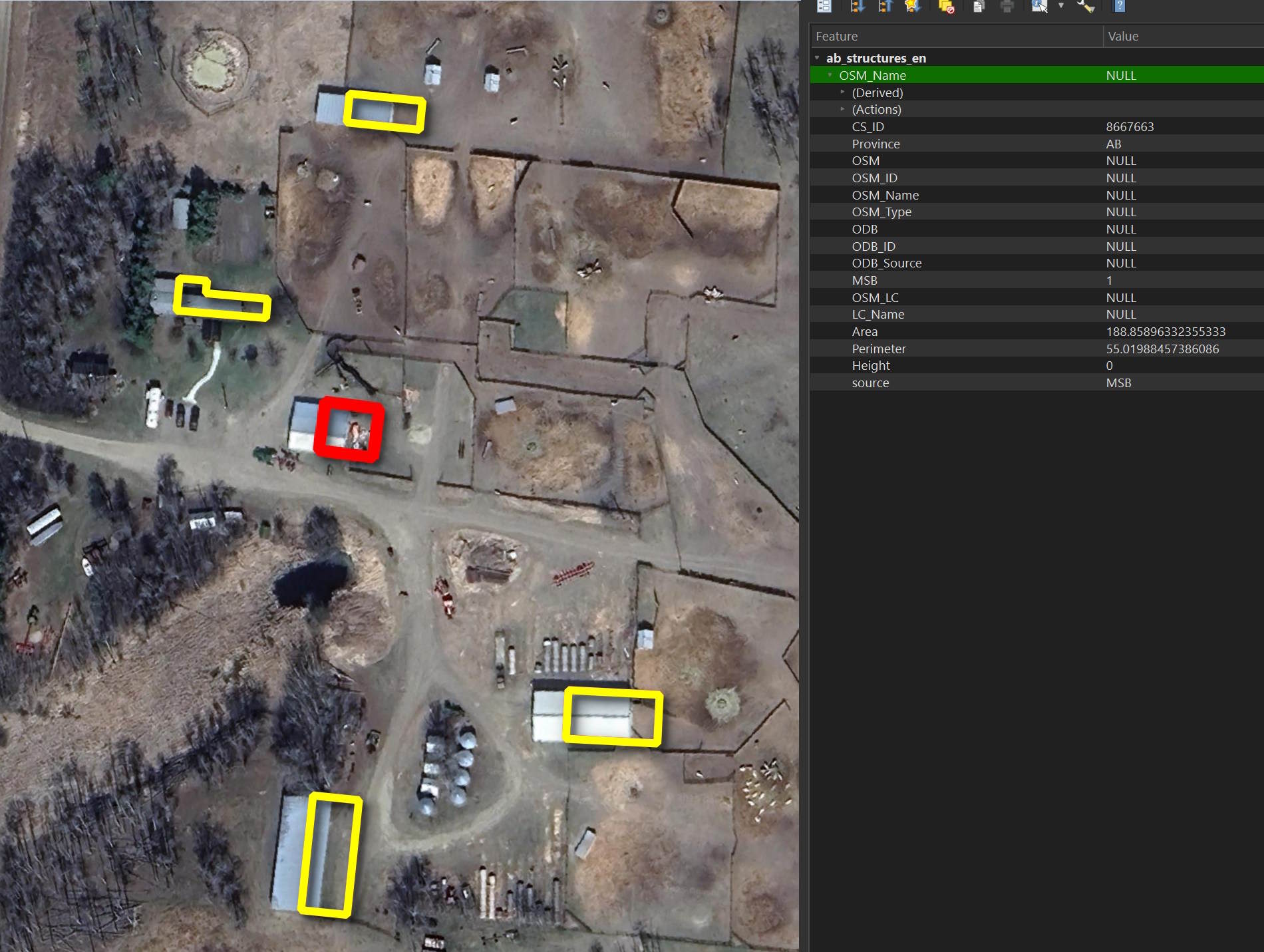
MSB footprints can take on a life of their own. Below is a screen shot from Northern Alberta.
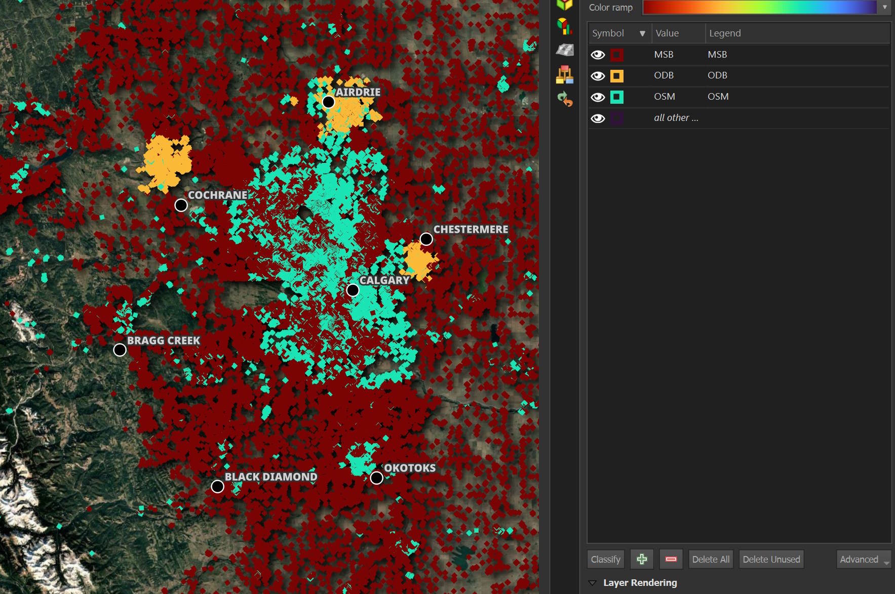
These are the sources of each footprint in PSC's dataset. It is a bit of a shame OSM wasn't picked as a first choice with ODB filling in the gaps.
I noticed Dease Lake, a remote community in Northern BC, has many of its homes, which have been on OSM since at least February 2023, missing.
Below are PSC's footprints in yellow on top of OSM's vector tiles for the area.
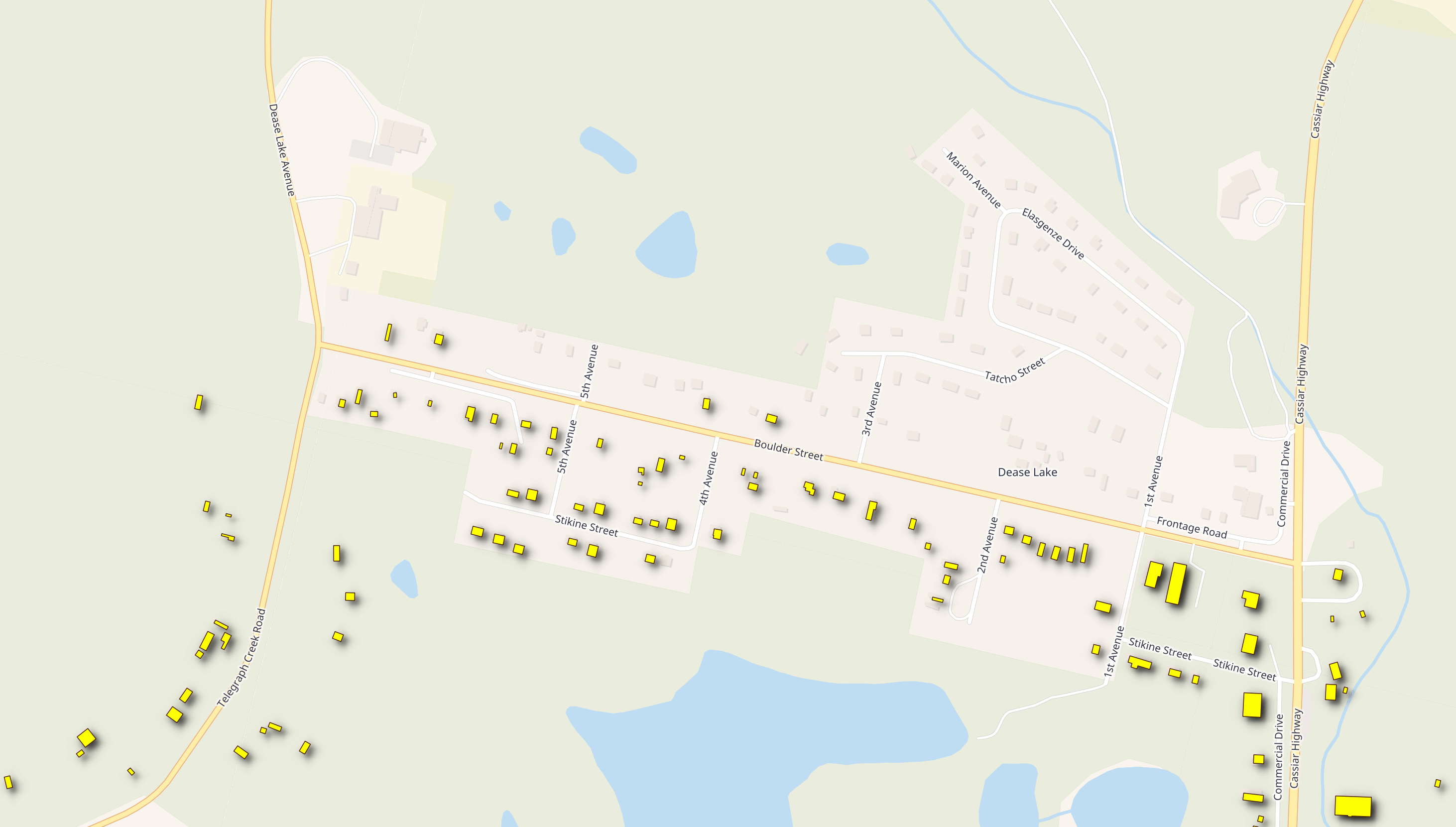
The following is one such example missing from PSC's dataset.
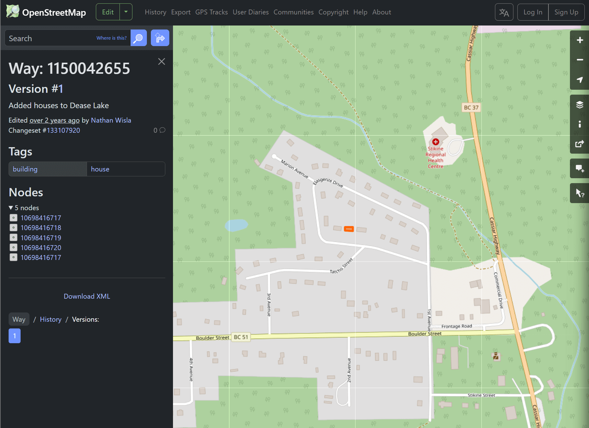
Provincial Boundaries
I looked along Alberta's borders with BC and SK and the provincial attributions to each of the buildings look very accurate.