Last Summer I published an Estonian Travel Guide aimed towards visitors making a first-time, 3-day journey. The maps in the guide were built largely with Estonian Land Board data and rendered in QGIS. I aimed to make the PDF small so that it could be downloaded on an unreliable internet connection and could be easily read off of a mobile phone.
Since then, I've been collecting research material for a trip to Tokyo I hope to make one day. I've been collecting points of interest (POIs) that I want to visit. I've also been coming up with some ideas of how to best render these on a map. My aims for this map are as follows:
- Plotting Points of Interest (POIs) that I have shorted listed.
- Road names in both English and Japanese.
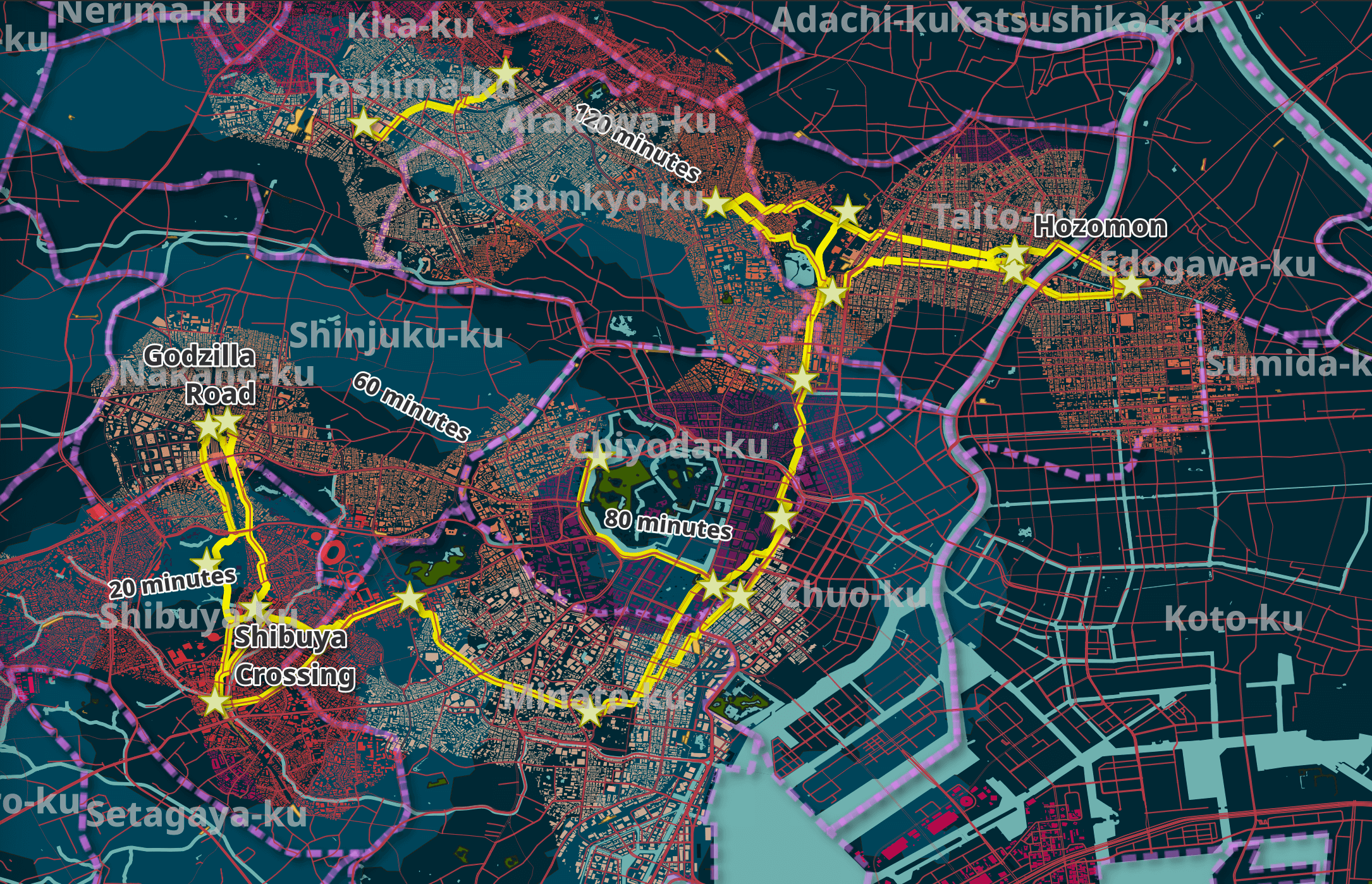
- Highlighting the shortest walking routes between any two POIs within 3 KM of one another.
- Render buildings around the walking routes and POIs. These should be colour-coded by the population density of the area.
- An isochrone showing how far it would take to walk from Shibuya Crossing to any point in the city within two hours. This should be partitioned into 20-minute increments.
Below is a rendering of my first attempt at putting this map together.

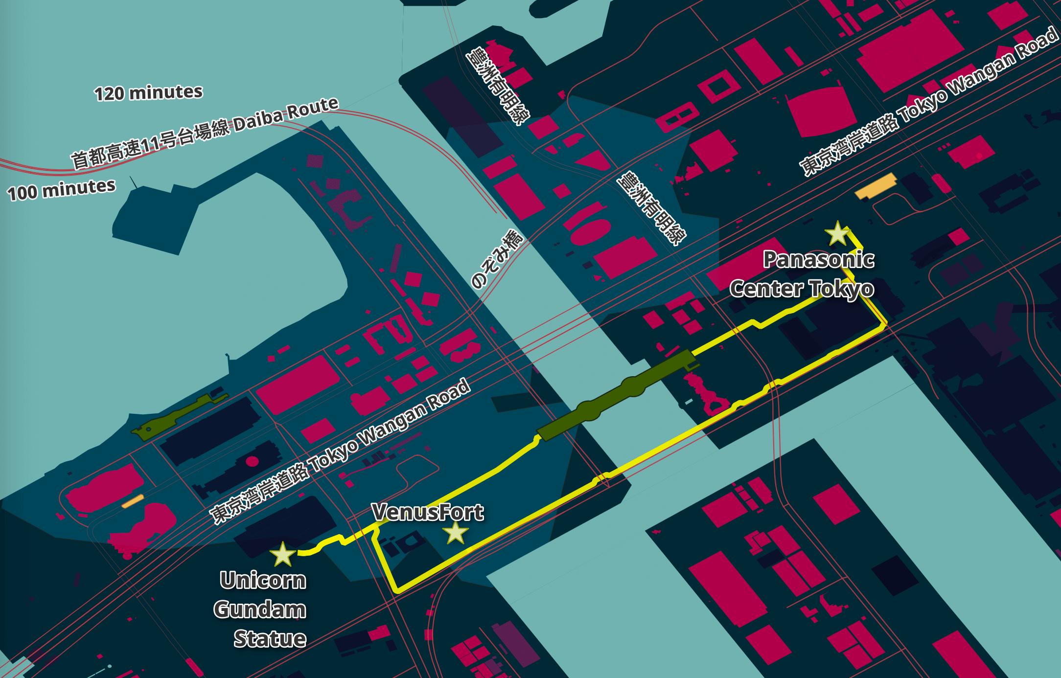
Below is a closer look at one section of the map.
In this blog post, I'll walk through the steps I took to produce this map. Please treat the material here as a work in progress. I couldn't consider a guide like this done until I've at least had the chance to use it in real life and iterate on it further.
Installing Prerequisites
The laptop I'm using is a 13" 2020 MacBook Pro running macOS 13.2.1. It has an Intel Core i5 quad-core locked at 1.4 GHz with a turbo boost speed of up to 3.9GHz, 8 GB of 2133 MHz LPDDR3 RAM, 250 GB of SSD capacity and an external 1 TB SSD that will store the GIS data used in this post.
I've installed Homebrew and I'll use it to install Python, DuckDB and a few other utilities.
$ brew install \
    awscli \
    duckdb \
    gdal \
    jq \
    virtualenv \
    wget
I'll use DuckDB's JSON, Parquet and Spatial extensions in this post.
$ duckdb
INSTALL json;
INSTALL spatial;
INSTALL parquet;
I'll set up DuckDB to load all these extensions each time it launches.
$ vi ~/.duckdbrc
.timer on
.width 180
LOAD json;
LOAD spatial;
LOAD parquet;
I'll then install my osm_split package which will be used to extract OpenStreetMap (OSM) features into named GeoPackage files.
$ virtualenv ~/.osm
$ source ~/.osm/bin/activate

$ git clone https://github.com/marklit/osm_split ~/osm_split
$ pip install -r ~/osm_split/requirements.txt
I'll also install a few more Python-based dependencies that will be used later on in this post.
$ pip install \
    polyline \
    rasterio \
    requests \
    xmltodict
The maps in this post were rendered with QGIS version 3.34. QGIS is a desktop application that runs on Windows, macOS and Linux. The software is very popular in the geospatial industry and was launched almost 15 million times in May last year.
I'll use QuickWKT to paste WKT strings from the command line into QGIS on a few occasions in this post.
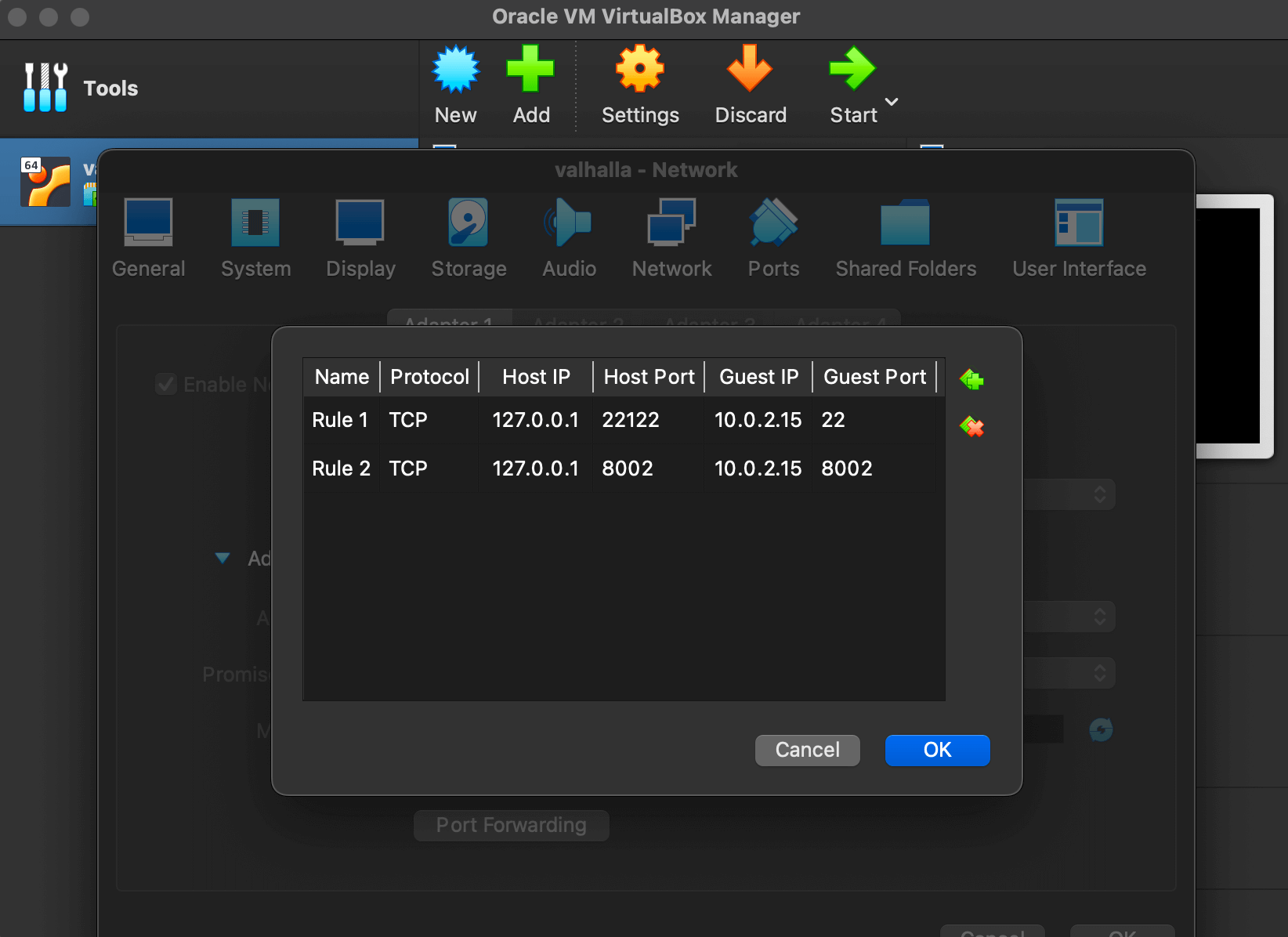
The routing calculations in this post will be handled by Valhalla. My Awesome Isochrones post explains how to install it. I used Ubuntu Server 22 running in a VirtualBox VM with 4 GB of RAM and 100 GB of storage space on my MacBook Pro. I set up port forwarding for TCP ports 22 and 8002 between my machine and 10.0.2.15 on the VM.
I made sure the VM and QGIS weren't both running at the same time to conserve as much of the 8 GB of RAM my machine has.
I've used Noto Sans as the sole font on this map. It does an amazing job of rendering both Latin and Japanese scripts.

Downloading Geospatial Datasets
I'll create a folder on an external SSD and download the latest 386 MB OSM extract for Japan's Kantō region, which includes the Tokyo Metropolitan Area.
$ mkdir -p /Volumes/Seagate/gis/Japan
$ cd /Volumes/Seagate/gis/Japan

$ wget https://download.geofabrik.de/asia/japan/kanto-latest.osm.pbf
The Overture Maps Foundation provides free global geospatial datasets. I covered their good work in a post last November. Their January release is around ~320 GB, 66% of which is dedicated to buildings. The buildings dataset has 320 Parquet files but the Tokyo building data can be found in just one of them. The following will download the 2 GB, ZStandard-compressed Parquet file of interest.
$ aws s3 cp --no-sign-request \
    s3://overturemaps-us-west-2/release/2024-01-17-alpha.0/theme\=buildings/type\=building/part-00046-cf0ca35a-8871-4c98-bfb8-13026efbae55-c000.zstd.parquet \
    ./overture_buildings_00046.pq
I'll be using a population density map of Tokyo to colour code the buildings on my map. The GeoTIFF containing this data is 1.7 GB in size.
$ unzip -j jpn-poppopmap15adj.zip
I used NASA's Earth at Night image as a basemap in one image. The 3600x1800 GeoTIFF version of this file is 4.6 MB.
Extracting OSM Features
The map's projection has been set to Japanese Geodetic Datum 2011 / EPSG:6668 which will make Japan look more like it would on a globe. All of the data fed into the map is in EPSG:4326 and QGIS takes care of the re-projection.
I'll create a folder to store the 1,374 GeoPackage files that will be created from OSM's Kantō region extract. There is a substantial amount of data within the OSM file and rendering all of it in QGIS would be extremely slow, even on my relatively new MacBook Pro. For this reason, I've found three H3 values covering the areas of Tokyo I'm interested in. If you haven't used H3 before, I wrote a post last September on how H3 geospatial indices work.
$ mkdir -p osm_20240120
$ cd osm_20240120

$ python3 ~/osm_split/main.py \
    ../kanto-latest.osm.pbf \
    --only-h3=842f5abffffffff,842f5a3ffffffff,842f5bdffffffff
The above produced 1.7 GB of GeoPackage data. Below are a few of the files produced.
$ ls -lht */electric*
2.8M ... points/electric_cables.gpkg
 97K ... multilinestrings/electric_cables.gpkg
 14M ... lines/electric_cables.gpkg
$ ls -lhS lines/building/ | head
143M ... house.gpkg
 24M ... apartments.gpkg
6.5M ... residential.gpkg
5.0M ... detached.gpkg
3.5M ... retail.gpkg
2.7M ... industrial.gpkg
2.2M ... commercial.gpkg
2.2M ... school.gpkg
1.1M ... greenhouse.gpkg
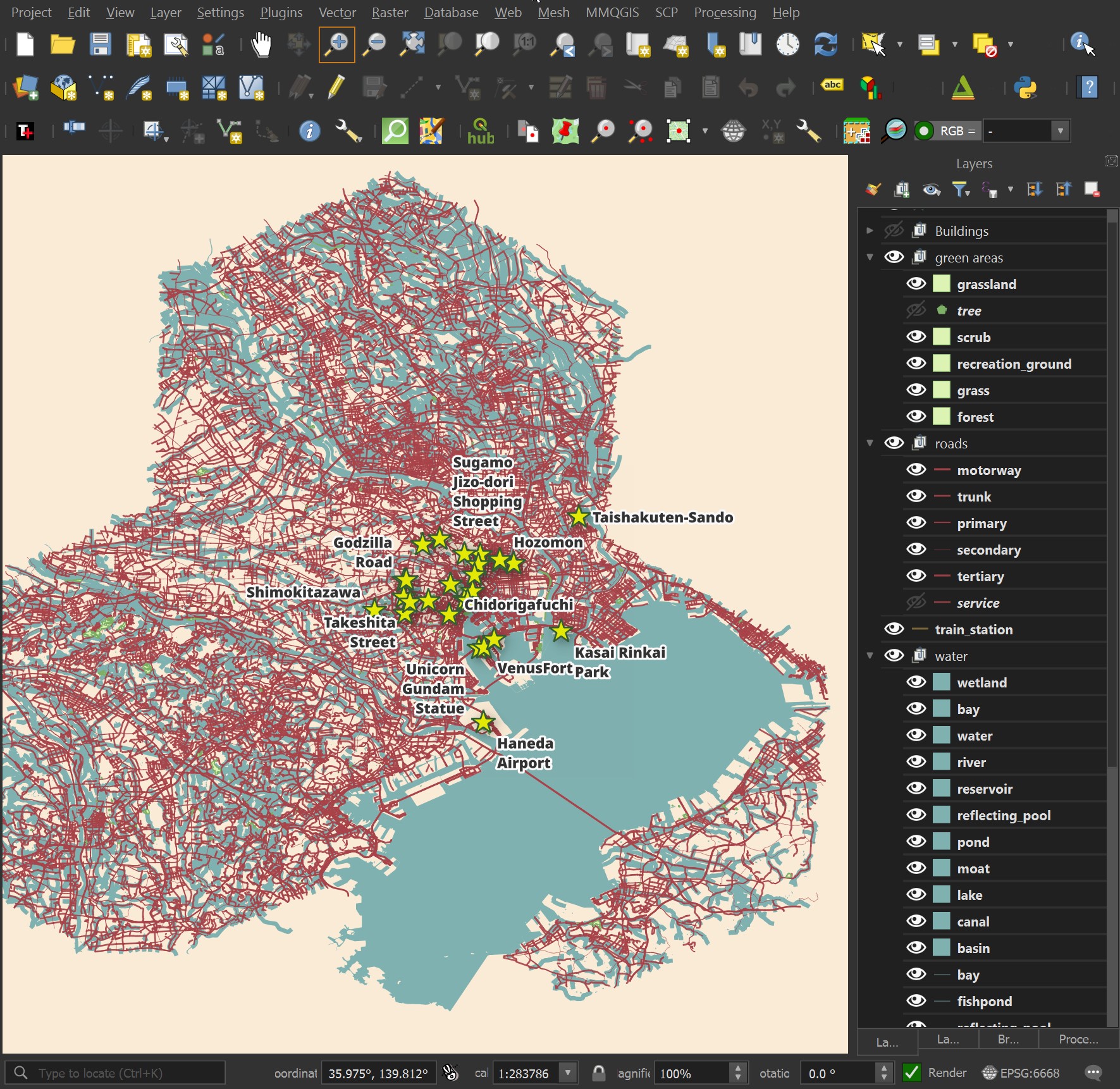
The following is a rendering of a few of the GeoPackage files. The outlines of the three hexagons show where the cut-off points were.
Tokyo's Streets
I've used the motorway, tertiary, trunk, primary and secondary road GeoPackage files. They're coloured #a84349 and have a line thickness of 0.4, 0.4, 0.3, 0.2 and 0.1 respectively.
I've concatenated their Japanese and English names together in 18-point labels that have 'Draw text buffer' enabled. Below is the QGIS formula for the labels.
CONCAT("name", ' ', "name:en")
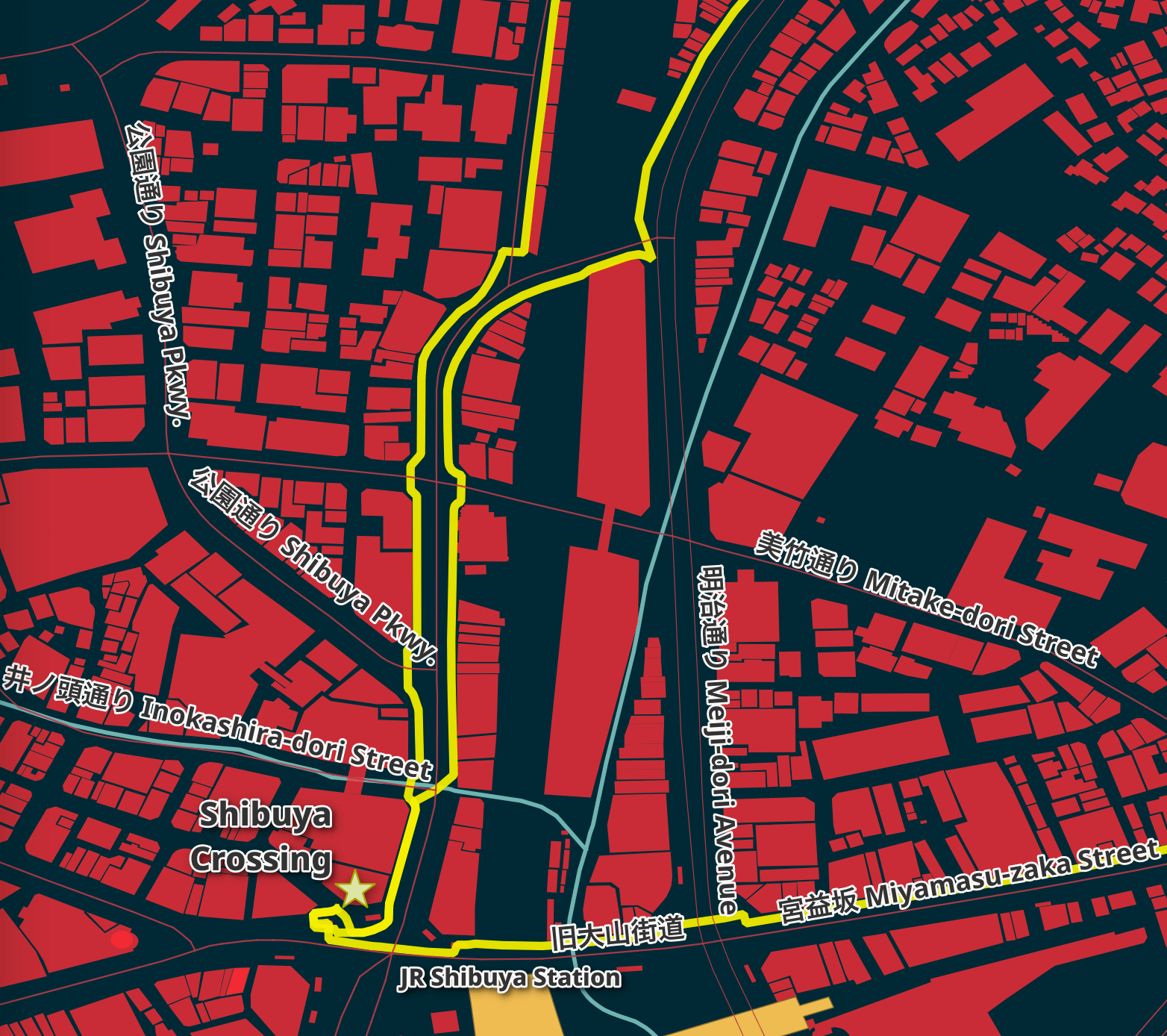
Japanese street names can be written using three different alphabets, even in a single word. Two of these alphabets have relatively simple symbols and I find them legible even with smaller font sizes.
The third alphabet, Kanji, contains 10s of thousands of characters and a single character can be made up of many strokes. In March of 2020, Taito was added to Unicode. It's made up of 84 strokes. It's complex and isn't easily legible when rendered with a small font size.
For this reason, I set the font size larger than I normally would as there is a fair amount of detail in these characters you'll need to see to match up to a street sign in real life.
Rivers & Green Areas
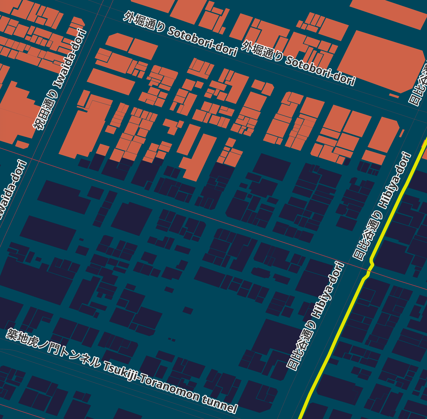
I used the grassland, scrub, recreation_ground, grass and forest polygon GeoPackage files for the green areas in the map. These are coloured #435c12 with a 0.4-point #1c2817 outline. This lay sits above all but the POIs layer.
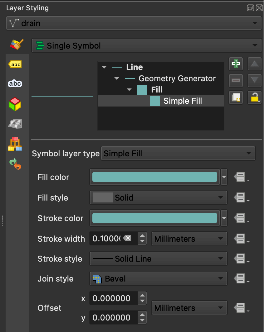
The water GeoPackage files are from both the multi-polygon and line folders. They're coloured #7fb1b0. The line strings use polygon geometry generation to fill in their interiors.
Points of Interest
I've pin-pointed 27 POIs in Tokyo using Google Earth and exported them to a KMZ file. The KMZ file is a ZIP file containing a doc.kml XML file. I'll extract out the POI names and their coordinates and print them out in CSV format. I'll then save that to a pois.csv file that I can then import into QGIS.
$ python3
import json
import zipfile

import xmltodict


pois = xmltodict.parse(
            zipfile.ZipFile('POI Inside Tokyo.kmz', 'r')
                   .open('doc.kml', 'r').read())

print('wkt,name')

for pm in pois['kml']['Document']['Folder']['Placemark']:
    print('"POINT(%s %s)","%s"' % (pm['LookAt']['longitude'],
                                   pm['LookAt']['latitude'],
                                   pm['name']))
This is the resulting CSV data.
wkt,name
"POINT(139.699325900317 35.67639759983872)","Meiji Jingu Shrine"
"POINT(139.7765215062398 35.71883513162575)","Tokyo National Museum"
"POINT(139.8107003999255 35.71006269989103)","Tokyo Skytree"
"POINT(139.7454329219986 35.65858058296164)","Tokyo Tower"
"POINT(139.7465035483471 35.68925215083959)","Chidorigafuchi"
"POINT(139.7606369001807 35.71984560025591)","Nezu Shrine"
"POINT(139.7003598206243 35.65984737050033)","Shibuya Crossing"
"POINT(139.7747151005004 35.70898599962936)","Ameyoko Shopping Street"
"POINT(139.6995725001277 35.69296140050677)","Omoide Yokocho"
"POINT(139.7964541999754 35.71184129989386)","Nakamise Shopping Street"
"POINT(139.858553400224 35.64134539964437)","Kasai Rinkai Park"
"POINT(139.6697139314947 35.66270699639875)","Shimokitazawa"
"POINT(139.7754916992781 35.62445100039961)","Unicorn Gundam Statue"
"POINT(139.7052180998863 35.67113509956779)","Takeshita Street"
"POINT(139.7798375749356 35.54939487023734)","Haneda Airport"
"POINT(139.7602977000509 35.67369979979083)","Godzilla Head"
"POINT(139.7237512209223 35.67226580092602)","Honda Welcome Plaza"
"POINT(139.8765617716076 35.75767468302779)","Taishakuten-Sando"
"POINT(139.7353669133122 35.73540490683516)","Sugamo Jizo-dori Shopping Street"
"POINT(139.7966332998452 35.71393329992739)","Hozomon"
"POINT(139.7181928121655 35.72938664301591)","Sky Circus Observatory"
"POINT(139.7685582006561 35.6820138002826)","Tokyo Character Street"
"POINT(139.7801640896117 35.62505867943557)","VenusFort"
"POINT(139.7905276000612 35.63315020022179)","Panasonic Center Tokyo"
"POINT(139.7635578282706 35.67247481220829)","Sony Building"
"POINT(139.7710645005295 35.69868950038415)","Sega Building Akihabara"
"POINT(139.701836392052 35.69367691234108)","Godzilla Road"
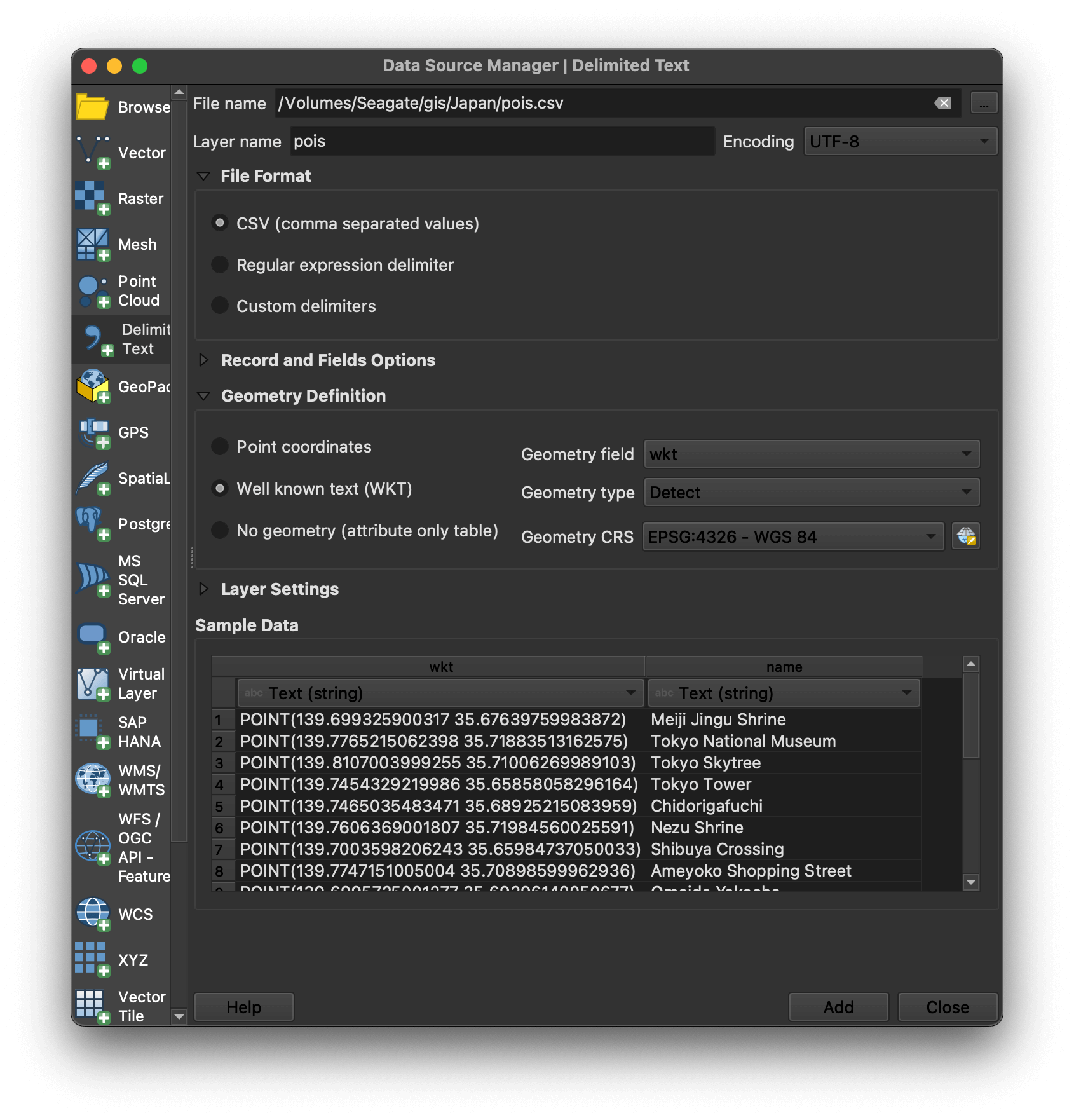
In QGIS, click the Layer Menu -> Add Layer -> Add Delimited Text Layer. Select pois.csv and make sure "Well known text (WKT)" is selected in the Geometry Definition section of the UI and wkt is selected as the Geometry field.
I've set the points' layer styling to use the star icon with a colour of #dfe4ac, size 10 and a solid #a4a422 stroke of 0.4.
The labels are using Noto Sans ExtraBold at 22 points in size with 'Draw text buffer' enabled. Below are three POIs rendered on the final map.

Walking Distances & Routes
I'll use Valhalla to produce a time-distance matrix between all 27 POIs.
import json
from   itertools import chain

import polyline
import requests


points = [{"lat": pm['LookAt']['latitude'],
           "lon": pm['LookAt']['longitude']}
          for pm in pois['kml']['Document']['Folder']['Placemark']]

tdm = json.loads(
        requests.post('http://127.0.0.1:8002/sources_to_targets',
                      json={'sources': points,
                            'targets': points,
                            'costing': 'pedestrian'}).content)
I'll then find every unique route that is less than 3 KM in length.
def sort_pairs(first, second):
    if first['lon'] < second['lon']:
        return (first['lat'], first['lon'],
                second['lat'], second['lon'])

    return (second['lat'], second['lon'],
            first['lat'], first['lon'])


pairs = set([sort_pairs(tdm['sources'][x['from_index']],
                        tdm['sources'][x['to_index']])
             for x in chain(*tdm['sources_to_targets'])
             if x['distance'] > 0.1
             and x['distance'] < 3])
I'll then get the line string data for each of these routes and convert them from polyline format into WKT before saving them into a CSV file. Each route will have multiple legs, with each of these legs being represented as its own WKT line string. As these routes are only for highlighting the streets one needs to walk on it's fine not to group them by route.
The polylines set will be used later on in the blog post.
def polyline_to_wkt(poly_line:str):
    return 'LINESTRING(%s)' % \
               ', '.join(['%f %f' % (lon, lat)
                          for lon, lat in polyline.decode(poly_line,
                                                          6,
                                                          geojson=True)])

legs, polylines = set(), set()

for lat1, lon1, lat2, lon2 in pairs:
    route = json.loads(
        requests.post('http://127.0.0.1:8002/route',
                      json={'costing': 'pedestrian',
                            'locations': [
                               {'lat': lat1, 'lon': lon1},
                               {'lat': lat2, 'lon': lon2}]}).content)

    for leg in route['trip']['legs']:
        polylines.add(leg['shape'])
        legs.add(polyline_to_wkt(leg['shape']))

with open('legs.csv', 'w') as f:
    f.write('wkt,\n')

    for leg in legs:
        f.write('"%s"\n' % leg)
I'll import legs.csv into QGIS as a new layer. The lines will be 2 points thick and coloured #f6f104. This layer is placed below the roads layers so it'll highlight routes rather than obstruct the existing roads. The roads layers contain the labels for the street names already.
The clusters of routes aren't completely connected as some of the clusters are more than 3 KM apart. I would expect when commuting between these clusters to find some sort of motorised transport between them rather than walk.
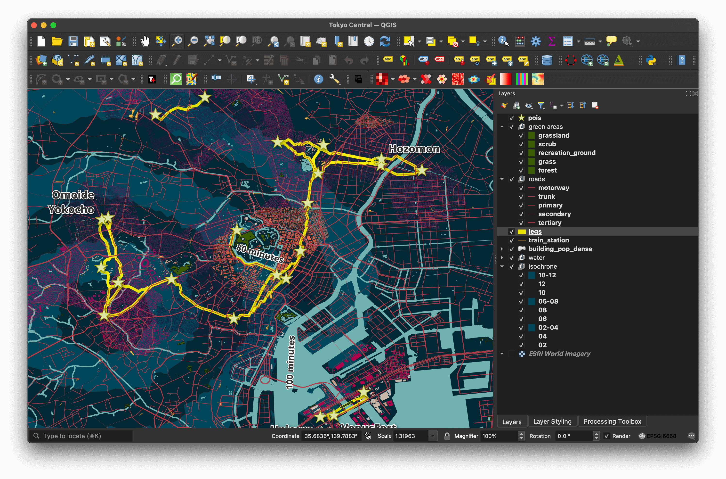
This shows the roads being highlighted by the shortest walking routes.

Tokyo's Building Footprints
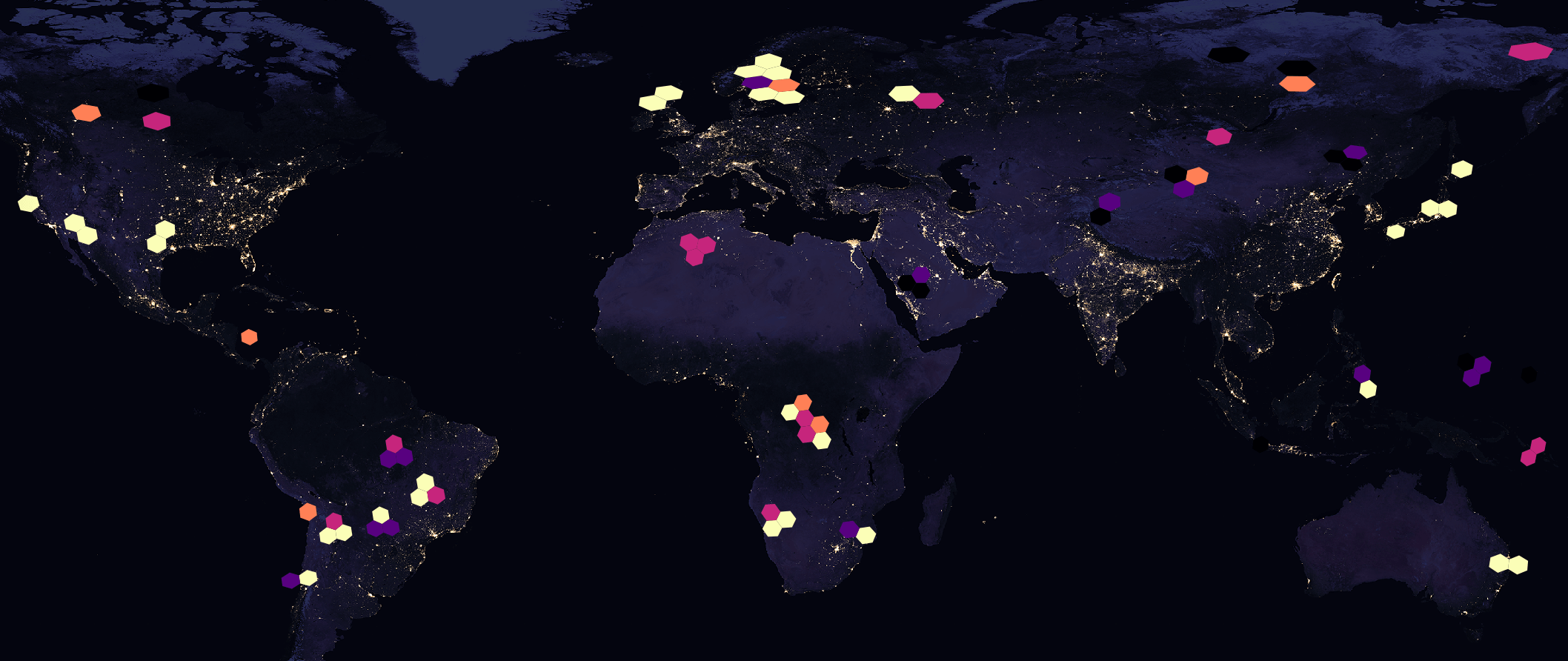
Overture Maps' January release contained ~212 GB of building footprint data spanning the Globe. Of the 320 PQ files used, only one contained data for the Tokyo Metropolitan Area. This file has 18,603,581 records, many of which do not relate to Tokyo. Below is a heatmap showing the locations of the buildings in this file.
I wrote the following to produce the WKT values for the three H3 hexagons around Tokyo that I'm interested in.
from h3 import h3_to_geo_boundary as get_poly

from shapely.geometry import Polygon


for h3_4 in ('842f5abffffffff',
             '842f5bdffffffff',
             '842f5a3ffffffff'):
    print(Polygon([[x, y] for x, y in get_poly(h3_4, geo_json=True)]))
I then used them to write a DuckDB SQL statement that would extract the building data from the Parquet file of interest. This statement will produce a centroid of every building and any that fall inside of one of the three hexagons will be included in the resulting table.
Side note: the H3 extension for DuckDB would have removed the need for the Python above and made the WHERE clause much shorter. If you're interested in using it instead I have a H3 geospatial indices blog post with compilation instructions.
$ duckdb tokyo_buildings.duckdb
CREATE OR REPLACE TABLE isolated AS
    SELECT * EXCLUDE (geometry,
                      bbox,
                      names,
                      sources),
           ST_GEOMFROMWKB(geometry) geom,
           ST_X(ST_CENTROID(geom)) centroid_x,
           ST_Y(ST_CENTROID(geom)) centroid_y,
           JSON(bbox)    AS bbox,
           JSON(names)   AS names,
           JSON(sources) AS sources
    FROM READ_PARQUET('overture_buildings_00046.pq')
    WHERE ST_WITHIN(ST_POINT(centroid_x, centroid_y)::POINT_2D,
                    ST_GeomFromText('POLYGON ((
                        140.11100565936707 35.36859420055637,
                        140.1263127801081 35.603627319068295,
                        139.9038543695014 35.736599553312075,
                        139.66734162397668 35.63425576574741,
                        139.65354890987163 35.399825444213576,
                        139.87475752025765 35.26713480800113,
                        140.11100565936707 35.36859420055637))')::POLYGON_2D)
    OR ST_WITHIN(ST_POINT(centroid_x, centroid_y)::POINT_2D,
                    ST_GeomFromText('POLYGON ((
                        139.65354890987163 35.399825444213576,
                        139.66734162397668 35.63425576574741,
                        139.44526000953354 35.76596883197294,
                        139.21064979075024 35.66298212531114,
                        139.19835841412598 35.4291674456274,
                        139.41917903778682 35.29772259518213,
                        139.65354890987163 35.399825444213576))')::POLYGON_2D)
    OR ST_WITHIN(ST_POINT(centroid_x, centroid_y)::POINT_2D,
                    ST_GeomFromText('POLYGON ((
                        139.9038543695014 35.736599553312075,
                        139.91854455148967 35.97153596077149,
                        139.69519602443003 36.10351941174491,
                        139.45842731845696 36.00029479199178,
                        139.44526000953354 35.76596883197294,
                        139.66734162397668 35.63425576574741,
                        139.9038543695014 35.736599553312075))')::POLYGON_2D);
The above matched 5,346,556 records out of the 18,603,581 in total. Five million polygons in QGIS will bring my machine to a halt.
Cutting Down the Search Space
I decided to find the zoom level 7 hexagons around every point of interest and route. I'll then extract the building data around these areas instead.
import zipfile

import h3
import polyline
import xmltodict


def polyline_to_h3(poly_line:str, zoom_level:int = 7):
    return set([h3.geo_to_h3(lat, lon, zoom_level)
                for lon, lat in polyline.decode(poly_line,
                                                6,
                                                geojson=True)])

h3_7s = set()

# polylines was produced earlier on in this post
for leg_shape in polylines:
    for h3_7 in polyline_to_h3(leg_shape):
        h3_7s.add(h3_7)

pois = xmltodict.parse(zipfile.ZipFile('POI Inside Tokyo.kmz', 'r')
                              .open('doc.kml', 'r').read())

for pm in pois['kml']['Document']['Folder']['Placemark']:
    h3_7s.add(h3.geo_to_h3(float(pm['LookAt']['latitude']),
                           float(pm['LookAt']['longitude']), 7))
The above produced 23 unique H3_7s. I'll build a DuckDB SQL statement to extract the buildings within these hexagons.
from  h3 import h3_to_geo_boundary as get_poly


def h3_to_wkt(h3_hex:str):
    return 'POLYGON((%s))' % \
               ', '.join(['%f %f' % (lon, lat)
                          for lon, lat in get_poly(h3_hex,
                                                   geo_json=True)])

where_clause = \
    ' OR '.join(["""ST_WITHIN(
                        ST_POINT(centroid_x, centroid_y)::POINT_2D,
                        ST_GeomFromText('%s')::POLYGON_2D)""" % h3_to_wkt(h3_7)
                 for h3_7 in h3_7s])

print('''COPY (
            SELECT * EXCLUDE (geometry,
                              bbox,
                              names,
                              sources),
                   ST_GEOMFROMWKB(geometry) geom,
                   ST_X(ST_CENTROID(geom)) centroid_x,
                   ST_Y(ST_CENTROID(geom)) centroid_y,
                   JSON(bbox)    AS bbox,
                   JSON(names)   AS names,
                   JSON(sources) AS sources
            FROM READ_PARQUET('overture_buildings_00046.pq')
            WHERE %s)
         TO 'tokyo_buildings.gpkg'
         WITH (FORMAT GDAL,
               DRIVER 'GPKG',
               LAYER_CREATION_OPTIONS 'WRITE_BBOX=YES')''' % where_clause)
I pasted the above SQL into DuckDB and a 201,105-record GeoPackage file was produced.
Population Density Enrichment
I'll iterate through each building of interest in the tokyo_buildings.gpkg file, find the population density value for their location and output that along with a WKT of the building's polygon into a CSV file.
$ python3
import json

import duckdb
import rasterio


def get_gpkg_record(gpkg_file: str):
    con = duckdb.connect(database=':memory:')
    con.execute('INSTALL spatial')
    con.execute('LOAD spatial')
    sql = """SELECT bbox,
                    ST_ASTEXT(geom)
             FROM ST_READ(?)"""

    res = con.sql(sql, params=(gpkg_file,))

    while True:
        rec = res.fetchone()

        if rec is None:
            return

        yield rec


with open('building_pop_dense.csv', 'w') as f:
    f.write('density,wkt\n')

    with rasterio.open('popmap15adj.tif') as population_map:
        for bbox, geom in get_gpkg_record('tokyo_buildings.gpkg'):
            bbox = json.loads(bbox)

            lon = (bbox['maxx'] - bbox['minx']) / 2 + bbox['minx']
            lat = (bbox['maxy'] - bbox['miny']) / 2 + bbox['miny']

            py, px  = population_map.index(lon, lat)
            window  = rasterio.windows.Window(px - 1 // 2,
                                              py - 1 // 2,
                                              1,
                                              1)
            clip    = population_map.read(window=window)
            density = int(clip[0][0][0])
            density = density if density > -1 and density < 1200 else 0
            f.write('%04d,"%s"\n' % (density, geom))
I'll use GDAL's ogr2ogr to convert the CSV file into a GeoPackage file. The GeoPackage version will load quicker and QGIS will maintain a higher frame rate when rendering it.
$ ogr2ogr \
    -f GPKG \
    building_pop_dense.gpkg \
    CSV:building_pop_dense.csv \
    -a_srs EPSG:4326
Below is a rendering of some of the buildings surrounded by the hexagons that were used for their selection.
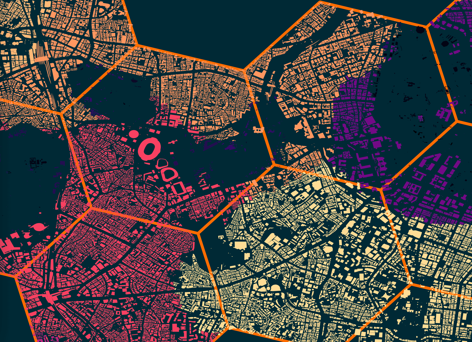
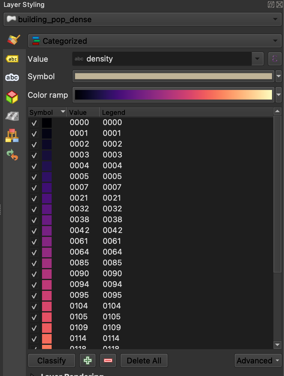
I used a colour ramp to colour each of the buildings based on their area's population density.
Route Finding
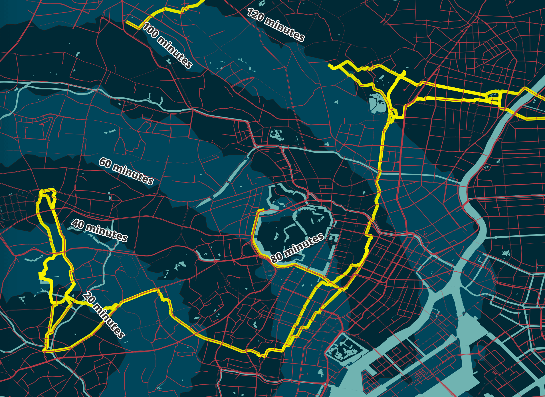
The map has three polygons that are shaded slightly brighter than the background and are used to show how long it would take to walk from Shibuya Crossing to the areas they cover. These are spread 20 minutes apart from one another.
I've used Valhalla to produce six polygon rings 20 minutes apart from one another.
$ python3
lat, lon = 35.65972, 139.70032

for minutes in (20, 40, 60, 80, 100, 120):
    iso = json.loads(
            requests.post('http://127.0.0.1:8002/isochrone',
                          json={'locations': [{'lat': lat,
                                               'lon': lon}],
                                'costing':   'pedestrian',
                                'contours':  [{'time': minutes}]}).content)
    print(Polygon(iso['features'][0]['geometry']['coordinates']).wkt)
I ran the above and pasted the resulting WKT strings into QGIS.
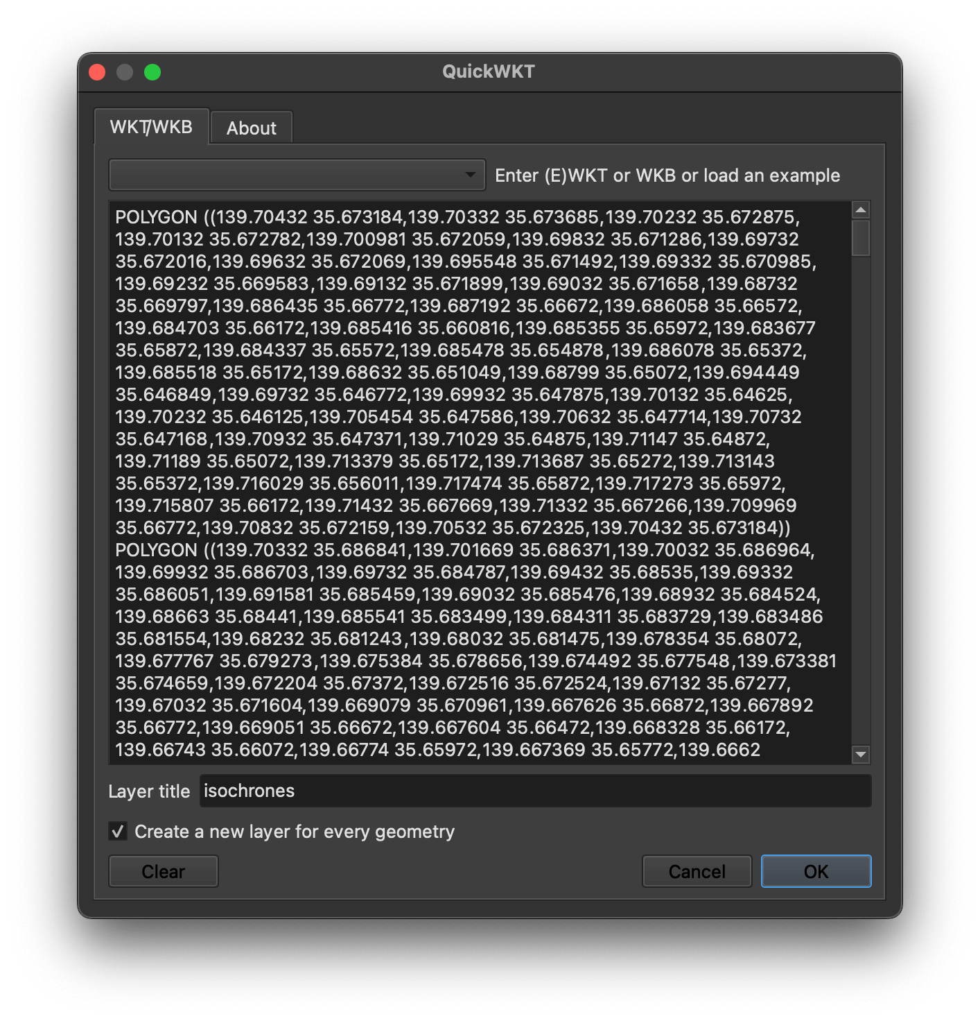
Then in QGIS, I clicked Vector Menu -> Geometry Tools -> Lines to Polygons on each of the six layers. This created new polygon versions of these layers. I subtracted the 20-minute polygon from the 40-minute polygon using Vector Menu -> Geoprocessing Tools -> Difference to create a hole in the 40-minute polygon. I then did the same for 80 and 60 minutes and 120 and 100 minutes.
The original isochrone layers were kept as well. I made their geometry transparent and used them for labelling each of the border areas.
The isochrone layers folder is the bottom folder in the project. The project's background colour is #032834 and the isochrone polygons are coloured #054559.
Ward Labels
When looking for taxi fare estimates, hotels or areas of interest, often places are referred to by the special ward that they are in. This appears to be administrative level 7 in Japan. Shibuya, Minato and Taitō are three examples.
I went through the administrative boundaries in OSM but I couldn't find any line strings or polygons which clearly identified all of these areas across Tokyo. Overture's Locality Area dataset did but it was missing names for these locations. I ended up finding a GitHub repo that contains GeoJSON for these areas, along with their names.
I've concatenated 63 GeoJSON files into a single file and dropped it into QGIS.
$ git clone https://github.com/utisz/compound-cities/
$ cd compound-cities
$ cat tokyo/*.json > wards.geojson
The styling needs polish but the wards are demarcated by dashed purple lines and the labels are 28-point Noto Sans Extra Bold coloured #bcbcbc with 70% opacity. This layer is above the water layer and below the buildings layer.
