I'm working on a reverse geocoder that uses Overture Maps' datasets. The prototype in this post can fetch the 2-letter ISO country code for any given point within a country's boundaries, return the nearest address and list countries within a given polygon.
My aim is to avoid paying API fees or making any network requests outside of the initial downloads of Overture's data.
In this post, I'll walk through this prototype and reverse geocode some satellite footprints.
My Workstation
I'm using a 5.7 GHz AMD Ryzen 9 9950X CPU. It has 16 cores and 32 threads and 1.2 MB of L1, 16 MB of L2 and 64 MB of L3 cache. It has a liquid cooler attached and is housed in a spacious, full-sized Cooler Master HAF 700 computer case.
The system has 96 GB of DDR5 RAM clocked at 4,800 MT/s and a 5th-generation, Crucial T700 4 TB NVMe M.2 SSD which can read at speeds up to 12,400 MB/s. There is a heatsink on the SSD to help keep its temperature down. This is my system's C drive.
The system is powered by a 1,200-watt, fully modular Corsair Power Supply and is sat on an ASRock X870E Nova 90 Motherboard.
I'm running Ubuntu 24 LTS via Microsoft's Ubuntu for Windows on Windows 11 Pro. In case you're wondering why I don't run a Linux-based desktop as my primary work environment, I'm still using an Nvidia GTX 1080 GPU which has better driver support on Windows and ArcGIS Pro only supports Windows natively.
Installing Prerequisites
I'll use Python 3.12.3 and jq to help analyse the data in this post.
$ sudo add-apt-repository ppa:deadsnakes/ppa
$ sudo apt update
$ sudo apt install \
    jq \
    python3-pip \
    python3.12-venv
Below, I'll set up a Python Virtual Environment and install some dependencies.
$ python3 -m venv ~/.overture_rcm
$ source ~/.overture_rcm/bin/activate
$ python3 -m pip install \
    awscli \
    duckdb \
    rich
I'll use DuckDB, along with its H3, JSON, Lindel, Parquet and Spatial extensions in this post.
$ cd ~
$ wget -c https://github.com/duckdb/duckdb/releases/download/v1.5.1/duckdb_cli-linux-amd64.zip
$ unzip -j duckdb_cli-linux-amd64.zip
$ chmod +x duckdb
$ ~/duckdb
INSTALL h3 FROM community;
INSTALL lindel FROM community;
INSTALL json;
INSTALL parquet;
INSTALL spatial;
I'll set up DuckDB to load every installed extension each time it launches.
$ vi ~/.duckdbrc
.timer on
.width 180
LOAD h3;
LOAD lindel;
LOAD json;
LOAD parquet;
LOAD spatial;
The maps in this post were rendered with QGIS version 4.0.1. QGIS is a desktop application that runs on Windows, macOS and Linux. The application has grown in popularity in recent years and has ~15M application launches from users all around the world each month.
I used QGIS' HCMGIS plugin to add basemaps from Bing and Esri to this post.
Overture's Divisions and Addresses
I did a deep dive comparing Overture's divisions with eleven other boundary datasets in December. Overture is tied in third place for most ISO country codes at 272 and has well-laid-out boundaries along coastlines.
These are their boundaries for Iceland. It's coloured by the boundary type with light blue for their land boundaries.
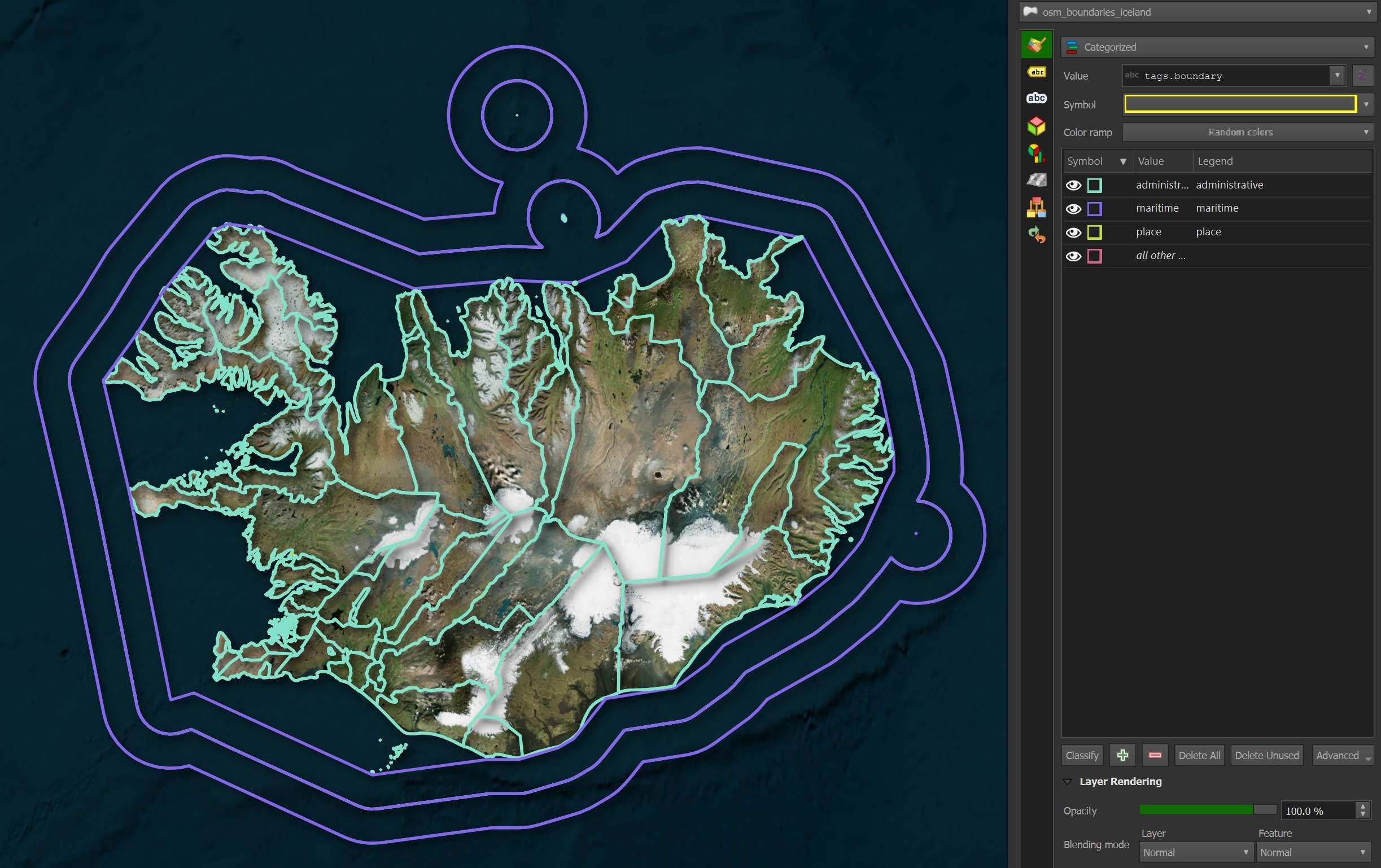
Most competing datasets did a poor job of hugging coastlines. Below are several examples for Bahrain.

I'll get this month's divisions dataset. The following downloaded 5.2 GB worth of Parquet files.
$ aws s3 --no-sign-request sync \
    s3://overturemaps-us-west-2/release/2026-04-15.0/theme=divisions/type=division_area/ \
    ~/division_area_2026-04-15.0
Overture's address dataset doesn't cover the globe but does have coverage for 39 countries as of this month's release. The following downloaded 21 GB worth of data.
$ aws s3 --no-sign-request sync \
    s3://overturemaps-us-west-2/release/2026-04-15.0/theme=addresses/type=address/ \
    ~/address_2026-04-15.0
Overture removes releases after 60 days. Use the following command to find out what the latest release is and replace the release string in the above URLs before trying to download anything.
$ aws s3 --no-sign-request ls \
    s3://overturemaps-us-west-2/release/
PRE 2026-03-18.0/
PRE 2026-04-15.0/
Reverse Geocoding in Python
I've put together three reverse geocoding functions.
The first takes a longitude and latitude pair and returns the nearest division's two-letter ISO country code. The list returned will contain an element that has a two-letter code. I'll likely refactor this to just return either a string in the future.
$ python3
import json

import duckdb
from   rich.progress import track


divisions = '/home/mark/division_area_2026-04-15.0/*.parquet'

con = duckdb.connect(database=':memory:')
con.sql('INSTALL spatial; LOAD spatial')

def nearest_iso2(lon:float, lat:float):
    fields = (
        'bbox',
        'class',
        'country',
        'division_id',
        'id',
        'is_land',
        'is_territorial',
        'names',
        'region',
        'sources',
        'subtype',
        'version')

    sql = '''SELECT %s
             FROM  '%s'
             ORDER BY ST_DISTANCE(
                        ST_POINT(bbox.xmin, bbox.ymin),
                        ST_POINT(%f, %f))
             LIMIT 1'''

    res = list(con.sql(sql % (','.join(fields),
                              divisions,
                              lon,
                              lat)).fetchall())

    return [{fields[num]: val
             for num, val in enumerate(rec)}
            for rec in res]
Below is an example result from a point in Tallinn, Estonia.
nearest_iso2(24.75294, 59.43412)
[{'bbox': {'xmin': 24.752965927124023,
   'xmax': 24.754074096679688,
   'ymin': 59.432708740234375,
   'ymax': 59.433204650878906},
  'class': 'land',
  'country': 'EE',
  'division_id': '18916d55-9bf3-4758-9691-83a462ec8204',
  'id': '89ee8bb5-8912-4d39-a8b9-487193cc9653',
  'is_land': True,
  'is_territorial': True,
  'names': {'primary': 'Islandi väljak', 'common': None, 'rules': None},
  'region': 'EE-37',
  'sources': [{'property': '',
    'dataset': 'OpenStreetMap',
    'license': 'ODbL-1.0',
    'record_id': 'w43735045@7',
    'update_time': '2024-02-14T15:13:23Z',
    'confidence': None,
    'between': None}],
  'subtype': 'microhood',
  'version': 1}]
The following will return a list of any country whose borders intersect a given polygon.
def countries_in_polygon(polygon:str):
    fields = (
        'id',
        'bbox',
        'country',
        'version',
        'sources',
        'subtype',
        'class',
        'names',
        'is_land',
        'is_territorial',
        'region',
        'division_id')

    sql = '''SELECT %s
             FROM '%s'
             WHERE country IN (
                SELECT DISTINCT country
                 FROM  '%s'
                 WHERE ST_Intersects(ST_POINT(bbox.xmin, bbox.ymin),
                                     '%s'::GEOMETRY)
                 LIMIT 100
             )
             AND subtype = 'country'
             AND class   = 'land'
             '''

    res = list(con.sql(sql % (','.join(fields),
                              divisions,
                              divisions,
                              polygon)).fetchall())

    return [{fields[num]: val
             for num, val in enumerate(rec)}
            for rec in res]
I've generated an example polygon shown below.
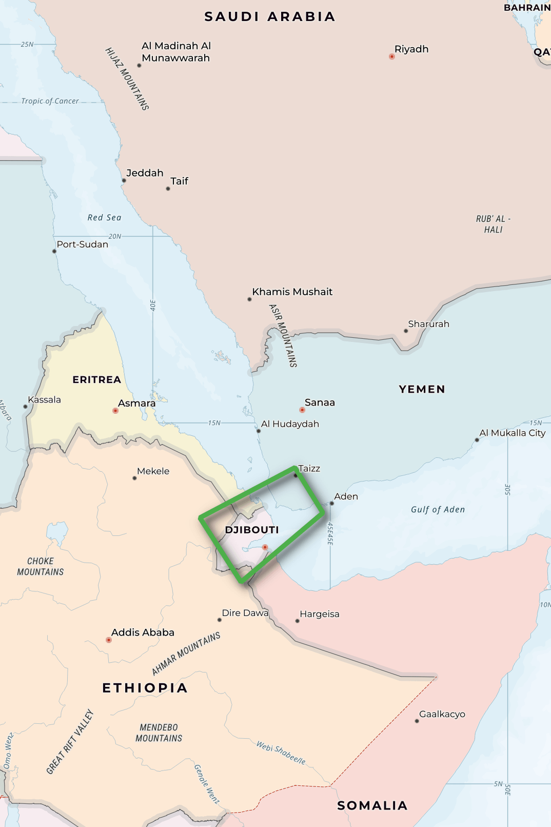
The following are the resulting matches.
res = countries_in_polygon('POLYGON ((41.32741049318353 12.40313010412833, 44.00517608732055 13.780566115995342, 44.79343608905786 12.53895263826337, 42.486616378091334 10.631257051879393, 41.32741049318353 12.40313010412833))')

print([(x['country'],
        x['names']['common']['en'])
       for x in res])
[('YE', 'Yemen'), ('ER', 'Eritrea'), ('DJ', 'Djibouti'), ('ET', 'Ethiopia')]
I'll need to use polygons for intersecting testing in the future as Somalia is missing from the results.
Below is a function that will return the nearest address to a given point. If the country is known ahead of time, this can be included as a predicate and will help minimise the search space. I've also added ranges around the longitude and latitude to help speed up the query. This is unlikely to be the fastest way to do a lookup and is still a work in progress.
addresses = '/home/mark/address_2026-04-15.0/*.parquet'


def nearest_address(lon:float, lat:float, countries:list=None):
    where = '''WHERE bbox.xmin > %f AND bbox.xmin < %f
               AND   bbox.ymin > %f AND bbox.ymin < %f''' % (
                    lon - 1, lon + 1,
                    lat - 1, lat + 1)

    if countries:
        where = where + ' AND country IN (%s)' % \
                        ','.join("'%s'" % x.upper()
                                 for x  in countries)

    fields = (
        'id',
        'street',
        'number',
        'unit',
        'postcode',
        'postal_city',
        'address_levels',
        'country',
        'sources',
        'version',
        'bbox',)

    sql = '''SELECT %s
             FROM  '%s'
             %s
             ORDER BY ST_DISTANCE(
                        ST_POINT(bbox.xmin, bbox.ymin),
                        ST_POINT(%f, %f))
             LIMIT 1'''

    res = list(con.sql(sql % (','.join(fields),
                              addresses,
                              where,
                              lon,
                              lat)).fetchall())

    return [{fields[num]: val
             for num, val in enumerate(rec)}
            for rec in res]
Below is an example from a point in Tallinn, Estonia.
nearest_address(24.75294, 59.43412, ['EE'])
[{'id': 'd054bf1b-05d7-4ebd-8e65-69aca6ea41fb',
  'street': 'Estonia puiestee',
  'number': '7',
  'unit': None,
  'postcode': None,
  'postal_city': None,
  'address_levels': [{'value': 'Harju maakond'},
   {'value': 'Tallinn'},
   {'value': 'Kesklinna linnaosa'}],
  'country': 'EE',
  'sources': [{'property': '',
    'dataset': 'OpenAddresses/MAA-AMET',
    'license': None,
    'record_id': None,
    'update_time': None,
    'confidence': None,
    'between': None}],
  'version': 1,
  'bbox': {'xmin': 24.752660751342773,
   'xmax': 24.75266456604004,
   'ymin': 59.434288024902344,
   'ymax': 59.434295654296875}}]
Canada's RADARSAT
Canada has been running a satellite programme called RADARSAT since the 1990s. The first constellation was launched in 1995, the second in 2007 and the third (RCM) in 2019.
The three satellites in the RCM constellation capture Synthetic Aperture Radar (SAR) imagery as well as AIS tracking data from ships. SAR allows for imagery to be taken day or night and can see through clouds and through some types of camouflage.
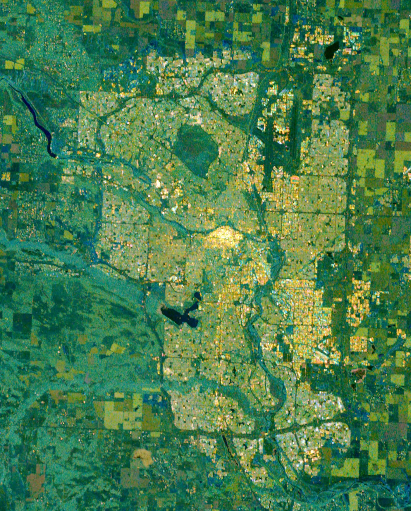
Below is a screenshot of a 96 GB, Cloud-Optimised GeoTIFF mosaic of RCM's imagery of Canada.
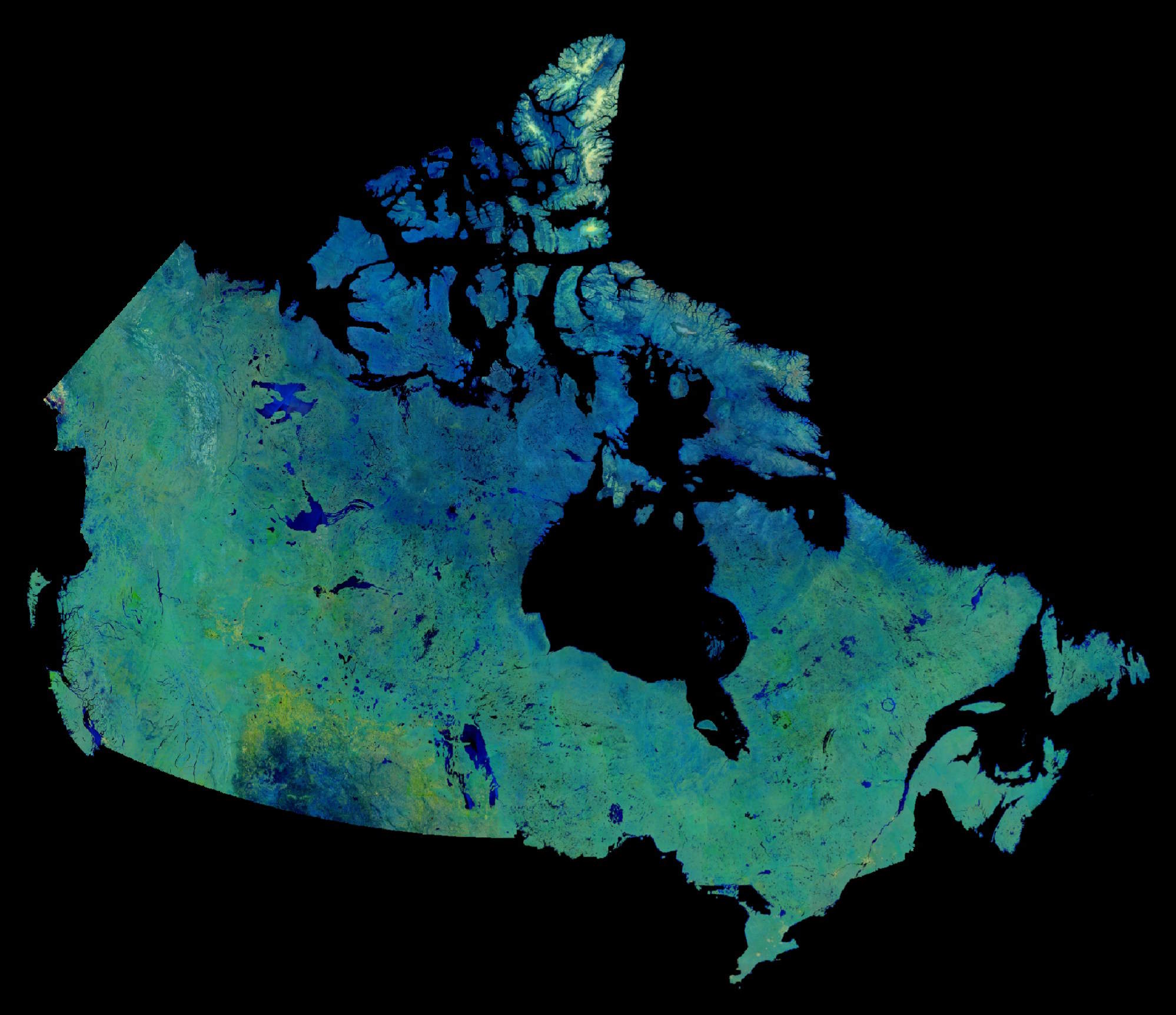
Below, I've zoomed into Calgary.
RADARSAT's Acquisition Plans
Natural Resources Canada publishes its RCM imagery capture plans every two weeks.
Below I've downloaded their plan for March 11th - 25th. Note, they don't version these files so the file you'd download will likely differ from the one I downloaded a few weeks ago.
$ wget https://ftp.maps.canada.ca/pub/csa_asc/Space-technology_Technologie-spatiale/radarsat_constellation_mission_plan/radarsat_constellation_mission_planned.shp.zip

$ unzip -j \
    -d radarsat_constellation_mission_planned \
    radarsat_constellation_mission_planned.shp.zip
I've cleaned up and converted their dataset into a Parquet file. There isn't a primary key in this dataset so I've added a UUID column. This will be used to join against other datasets later on in this post.
$ ~/duckdb
COPY(
    SELECT   baq:       BAQ,
             beam_id:   BEAMID,
             beam_type: BEAMTYPE_E,
             ccd:       CCD_E::BOOL,
             ccd_exact: EXACTCCD_E::BOOL,
             pol_type:  POLTYPE_E,
             prod_type: PRODTYPE_E,
             radar_md:  RADARMD,
             rx_pol:    RXPOL,
             sat_id:    SATID,
             tx_pol:    TXPOL,
             start_at:  UTC_STRT::TIMESTAMP,
             end_at:    UTC_END::TIMESTAMP,
             geometry:  geom,
             bbox:      {'xmin': ST_XMIN(ST_EXTENT(geom)),
                         'ymin': ST_YMIN(ST_EXTENT(geom)),
                         'xmax': ST_XMAX(ST_EXTENT(geom)),
                         'ymax': ST_YMAX(ST_EXTENT(geom))},
             uuid:      UUID()
    FROM     ST_READ('radarsat_constellation_mission_planned/radarsat_constellation_mission_planned.shx')
    ORDER BY HILBERT_ENCODE([ST_Y(ST_CENTROID(geom)),
                             ST_X(ST_CENTROID(geom))]::double[2])
) TO 'planned.parquet' (
  FORMAT 'PARQUET',
  CODEC  'ZSTD',
  COMPRESSION_LEVEL 22,
  ROW_GROUP_SIZE 15000);
The above produced a 3.1 MB Parquet file containing 4,911 rows.
Below is a breakdown of unique values and NULL coverage across each column.
SELECT   column_name,
         column_type[:30],
         null_percentage,
         approx_unique,
         min[:30],
         max[:30]
FROM     (SUMMARIZE
          FROM 'planned.parquet')
ORDER BY LOWER(column_name);
┌─────────────┬────────────────────────────────┬─────────────────┬───────────────┬────────────────────────────────┬────────────────────────────────┐
│ column_name │        column_type[:30]        │ null_percentage │ approx_unique │            min[:30]            │            max[:30]            │
│   varchar   │            varchar             │  decimal(9,2)   │     int64     │            varchar             │            varchar             │
├─────────────┼────────────────────────────────┼─────────────────┼───────────────┼────────────────────────────────┼────────────────────────────────┤
│ baq         │ VARCHAR                        │            0.00 │             3 │ 1 bit                          │ 3 bit                          │
│ bbox        │ STRUCT(xmin DOUBLE, ymin DOUBL │            0.00 │          5222 │ {'xmin': -180.0, 'ymin': -16.8 │ {'xmin': 177.82678, 'ymin': -1 │
│ beam_id     │ VARCHAR                        │            0.00 │           133 │ 16M10                          │ SCSDA                          │
│ beam_type   │ VARCHAR                        │            0.00 │            10 │ High Resolution 5m             │ Very High Resolution 3m        │
│ ccd         │ BOOLEAN                        │            0.00 │             2 │ false                          │ true                           │
│ ccd_exact   │ BOOLEAN                        │            0.00 │             2 │ false                          │ true                           │
│ end_at      │ TIMESTAMP                      │            0.00 │          4648 │ 2026-03-11 03:11:52            │ 2026-03-25 23:55:24            │
│ geometry    │ GEOMETRY('EPSG:4326')          │            0.00 │          4866 │ POLYGON ((-47.79754 44.06532,  │ MULTIPOLYGON (((-165.64809 74. │
│ pol_type    │ VARCHAR                        │            0.00 │             5 │ Compact Polarization           │ Single Polarization            │
│ prod_type   │ VARCHAR                        │            0.00 │             6 │ GRD - 16bit                    │ null - 32bit                   │
│ radar_md    │ VARCHAR                        │            0.00 │             3 │ ScanSAR                        │ Stripmap Continuous            │
│ rx_pol      │ VARCHAR                        │            0.00 │             3 │ H                              │ V                              │
│ sat_id      │ VARCHAR                        │            0.00 │             3 │ RCM-1                          │ RCM-3                          │
│ start_at    │ TIMESTAMP                      │            0.00 │          4306 │ 2026-03-11 03:09:27            │ 2026-03-25 23:55:17            │
│ tx_pol      │ VARCHAR                        │            0.00 │             4 │ C                              │ V                              │
│ uuid        │ UUID                           │            0.00 │          4543 │ 0017484c-9210-4479-935c-dec8bf │ fffe46dc-6588-429f-9787-eacafa │
└─────────────┴────────────────────────────────┴─────────────────┴───────────────┴────────────────────────────────┴────────────────────────────────┘
This is a rendering of the above dataset's footprints.
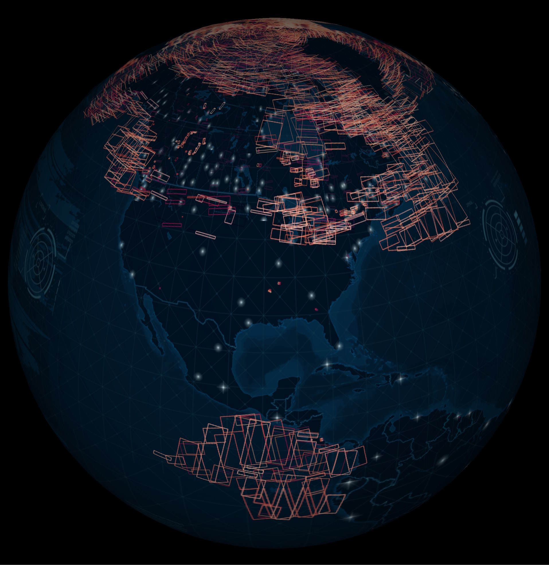
Below is an animation of the imagery capture plan. I've coloured every footprint by its date and used the temporal functionality in QGIS to render them by the hour they're captured.
Footprint Enrichment
I'll take every footprint in the RCM capture plan and run them through the reverse geocoding functions. The following produced a 72 MB, 4,911-line JSON file.
sql = '''SELECT uuid,
                geometry::TEXT,
                ST_X(ST_CENTROID(geometry)),
                ST_Y(ST_CENTROID(geometry)),
         FROM   'planned.parquet'
      '''

with open('planned.enriched.json', 'w') as f:
    for (uuid_, wkt, lon, lat) in track(list(con.sql(sql).fetchall())):
        nearest_iso2_ = nearest_iso2(lon, lat)
        countries_in_polygon_ = countries_in_polygon(wkt)

        f.write(json.dumps({
                    'uuid':                 uuid_,
                    'nearest_iso2':         nearest_iso2_,
                    'countries_in_polygon': countries_in_polygon_,
                    'nearest_address':
                        nearest_address(lon,
                                        lat,
                                        [x['country']
                                         for x in countries_in_polygon_])
                    },
                    sort_keys=True,
                    default=str) + '\n')
The above took a few hours to complete. I was hoping it would take a few minutes. I'm going to have to look into optimising this further in order to reach that performance target.
I'll create an enriched Parquet file that joins the above lookups with the acquisition plan dataset.
$ ~/duckdb
COPY(
    SELECT a.*,
           b.* EXCLUDE(uuid),
           nearest_country: b.nearest_iso2[1].country
    FROM   'planned.parquet' a
    JOIN   'planned.enriched.json' b ON a.uuid = b.uuid
) TO 'planned.enriched.parquet' (
  FORMAT 'PARQUET',
  CODEC  'ZSTD',
  COMPRESSION_LEVEL 22,
  ROW_GROUP_SIZE 15000);
The above produced a 3.7 MB Parquet file.
Below is an example record. I've truncated the names and sources lists as they're quite lengthy.
$ echo "FROM 'planned.enriched.parquet'
        LIMIT 1" \
    | ~/duckdb -json \
    | jq -S .
[
  {
    "baq": "3 bit",
    "bbox": {
      "xmax": -112.45445,
      "xmin": -116.8121,
      "ymax": 43.57581,
      "ymin": 42.57175
    },
    "beam_id": "SCLNB",
    "beam_type": "Low Noise",
    "ccd": "false",
    "ccd_exact": "false",
    "countries_in_polygon": [
      {
        "bbox": {
          "xmax": 179.7726287841797,
          "xmin": -179.14785766601562,
          "ymax": 71.38683319091797,
          "ymin": 18.91116714477539
        },
        "class": "land",
        "country": "US",
        "division_id": "f39eb4af-5206-481b-b19e-bd784ded3f05",
        "id": "79d2f02b-59b9-4981-8c88-43f07431788b",
        "is_land": true,
        "is_territorial": false,
        "names": {
          "common": {
            "en": "United States",
            ...
          },
          "primary": "United States of America",
          "rules": [...]
        },
        "region": null,
        "sources": [...],
        "subtype": "country",
        "version": 4
      }
    ],
    "end_at": "2026-03-11 13:46:18",
    "geometry": "POLYGON ((-112.45445 43.04819, -112.46727 43.00002, -112.48336 42.93853, -112.49843 42.87689, -112.51336 42.81523, -112.52955 42.75376, -112.54715 42.69249, -112.5631 42.63098, -112.57883 42.57175, -113.98181 42.76447, -115.39313 42.9399, -116.8121 43.09782, -116.80517 43.15753, -116.79738 43.2194, -116.78634 43.28094, -116.77776 43.34273, -116.76946 43.40456, -116.76037 43.46629, -116.74823 43.52771, -116.7382 43.57581, -115.30216 43.41781, -113.87399 43.24186, -112.45445 43.04819))",
    "nearest_address": [
      {
        "address_levels": [
          {
            "value": "ID"
          },
          {
            "value": null
          }
        ],
        "bbox": {
          "xmax": -114.61167907714844,
          "xmin": -114.6116943359375,
          "ymax": 43.03421401977539,
          "ymin": 43.03420639038086
        },
        "country": "US",
        "id": "fa6e6168-4ed2-4207-b268-7629f86f5e6e",
        "number": "2414",
        "postal_city": null,
        "postcode": "83314",
        "sources": [
          {
            "between": null,
            "confidence": null,
            "dataset": "NAD",
            "license": null,
            "property": "",
            "record_id": null,
            "update_time": null
          }
        ],
        "street": "East 1150 South",
        "unit": null,
        "version": 1
      }
    ],
    "nearest_country": "US",
    "nearest_iso2": [
      {
        "bbox": {
          "xmax": -114.69801330566406,
          "xmin": -114.7276382446289,
          "ymax": 42.94951629638672,
          "ymin": 42.91918182373047
        },
        "class": "land",
        "country": "US",
        "division_id": "2f9add0b-97fb-45cd-844e-017882674973",
        "id": "39c72352-3cdc-4bec-8221-67d5e347a2ca",
        "is_land": true,
        "is_territorial": true,
        "names": {
          "common": null,
          "primary": "Gooding",
          "rules": null
        },
        "region": "US-ID",
        "sources": [
          {
            "between": null,
            "confidence": null,
            "dataset": "OpenStreetMap",
            "license": "ODbL-1.0",
            "property": "",
            "record_id": "r121376@4",
            "update_time": "2020-12-11 20:02:43"
          }
        ],
        "subtype": "locality",
        "version": 1
      }
    ],
    "pol_type": "Dual Co/Cross Polarization",
    "prod_type": "GRD - 16bit",
    "radar_md": "ScanSAR",
    "rx_pol": "H+V",
    "sat_id": "RCM-3",
    "start_at": "2026-03-11 13:46:08",
    "tx_pol": "H",
    "uuid": "03e63006-456d-4fc3-92eb-40b0ee1535c6"
  }
]
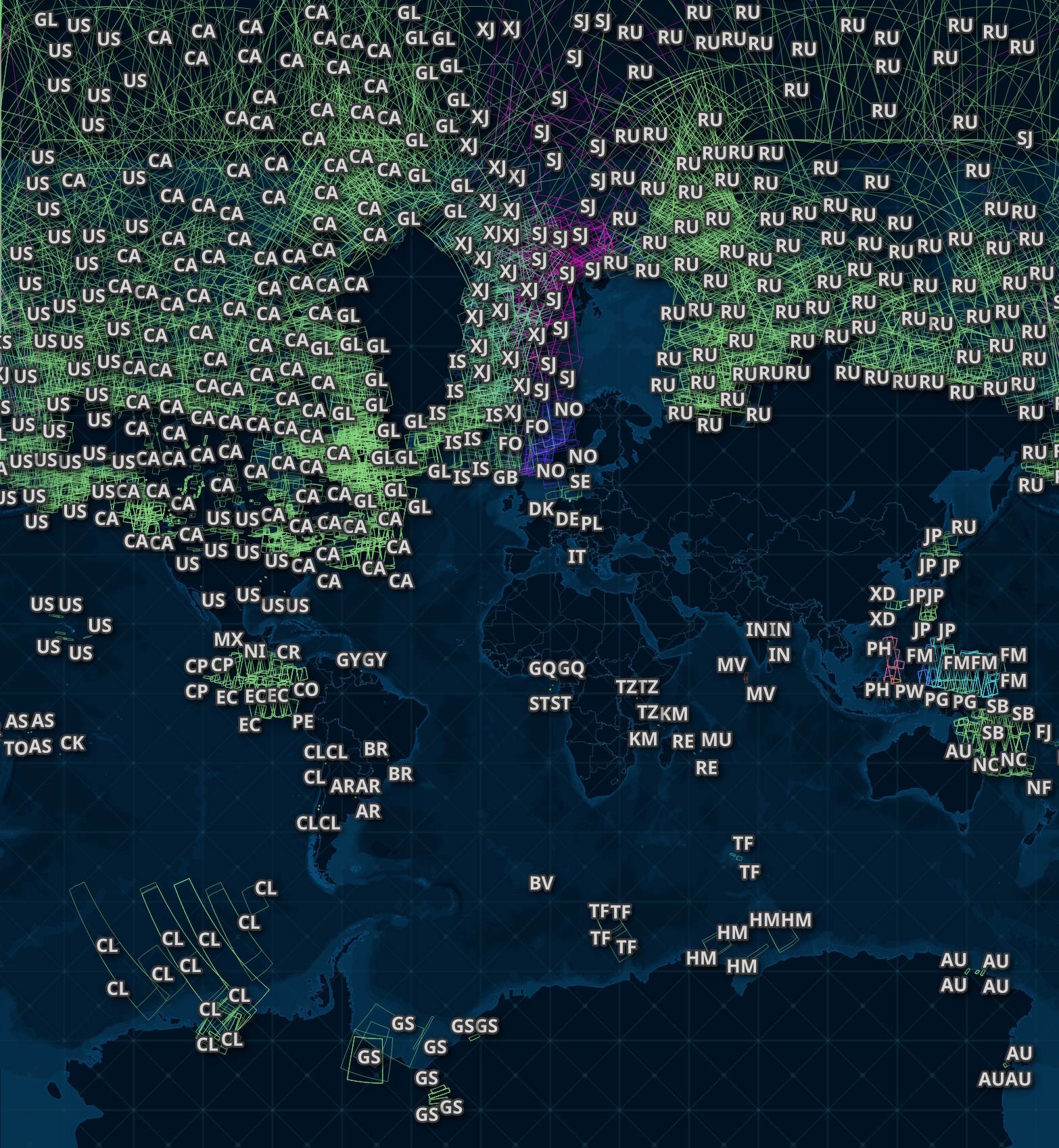
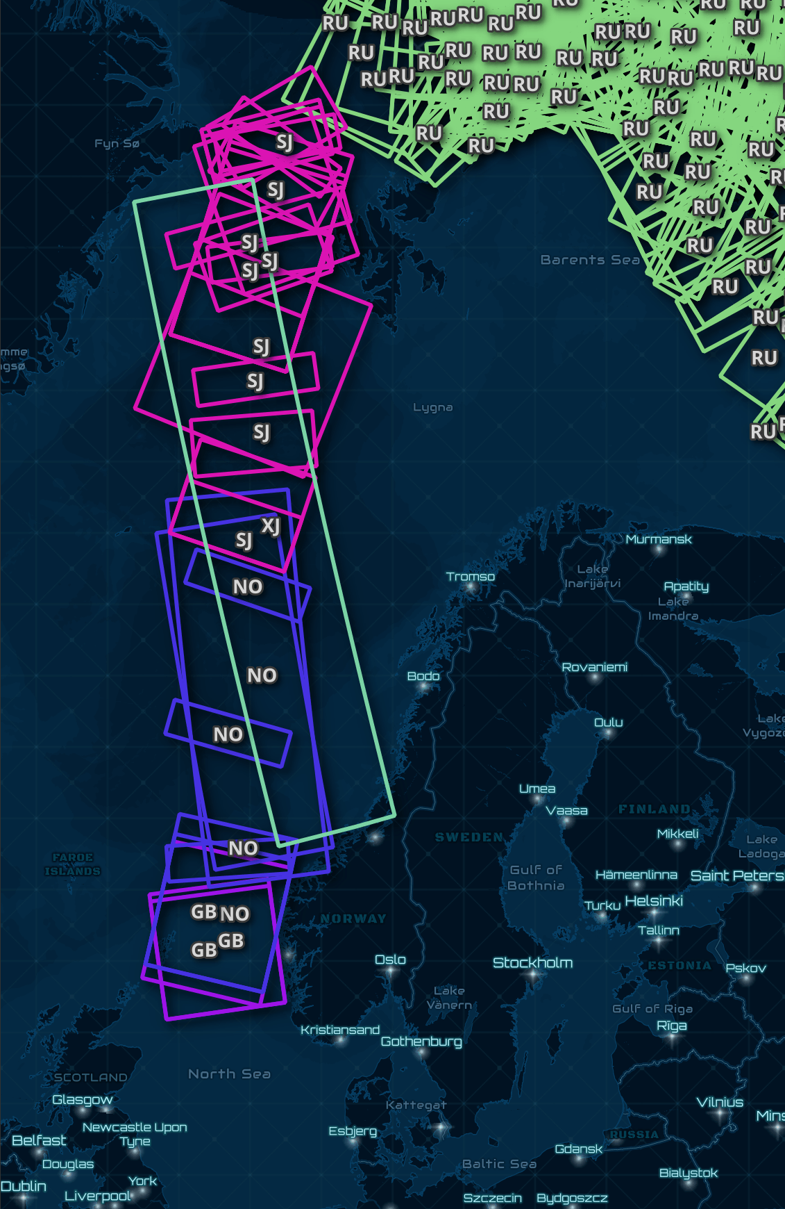
Below are some of the planned footprints between Greenland and Scandinavia. I've labelled each footprint with the nearest ISO2 country code in Overture's dataset. This image was taken while the above enrichment job was still running so there aren't as many footprints as in the final dataset.
A number of the footprints were over open oceans and wouldn't intersect with any country's boundaries. Below is a breakdown of the footprints with at least one country intersecting its footprint.
SELECT   has_intersection: LENGTH(countries_in_polygon) > 0,
         COUNT(*)
FROM     'planned.enriched.parquet'
GROUP BY 1;
┌──────────────────┬──────────────┐
│ has_intersection │ count_star() │
│     boolean      │    int64     │
├──────────────────┼──────────────┤
│ true             │         1794 │
│ false            │         3117 │
└──────────────────┴──────────────┘
If a footprint's nearest country isn't supported by Overture's address dataset and/or there are no addresses +/- 1 degree of latitude or longitude from the point given, then no address will be returned. Below is the breakdown of how many footprints have a nearest address.
SELECT   has_address: LENGTH(nearest_address) > 0,
         COUNT(*)
FROM     'planned.enriched.parquet'
GROUP BY 1;
┌─────────────┬──────────────┐
│ has_address │ count_star() │
│   boolean   │    int64     │
├─────────────┼──────────────┤
│ false       │         4032 │
│ true        │          879 │
└─────────────┴──────────────┘
Below are the footprint's most common nearest countries.
CREATE OR REPLACE TABLE country_names AS
    WITH b AS (
        WITH a AS (
            SELECT   country,
                     names.common.en,
                     area: ST_AREA(geometry)
            FROM     '/home/mark/division_area_2026-04-15.0/*.parquet'
            WHERE    names.common.en IS NOT NULL
        )
        SELECT *,
               ROW_NUMBER() OVER (PARTITION BY country
                                  ORDER BY     area DESC) AS rn
        FROM   a
    )
    FROM     b
    WHERE    rn = 1
    ORDER BY area DESC;

SELECT    num_footprints: COUNT(*),
          nearest_country,
          country_name: SPLIT_PART(en, '/', 1)
FROM      'planned.enriched.parquet'
LEFT JOIN country_names ON (nearest_country = country)
GROUP BY  2, 3
ORDER BY  1 DESC
LIMIT     20;
┌────────────────┬─────────────────┬──────────────────────────────────────────┐
│ num_footprints │ nearest_country │               country_name               │
│     int64      │     varchar     │                 varchar                  │
├────────────────┼─────────────────┼──────────────────────────────────────────┤
│           1868 │ CA              │ Canada                                   │
│            903 │ RU              │ Russia                                   │
│            589 │ US              │ United States                            │
│            405 │ GL              │ Greenland                                │
│            181 │ XJ              │ Jan Mayen                                │
│            102 │ SJ              │ Svalbard                                 │
│             98 │ IS              │ Iceland                                  │
│             69 │ FM              │ Federated States of Micronesia           │
│             61 │ CL              │ Chile                                    │
│             59 │ EC              │ Ecuador                                  │
│             47 │ NO              │ Norway                                   │
│             46 │ JP              │ Japan                                    │
│             45 │ AU              │ Australia                                │
│             42 │ PG              │ Papua New Guinea                         │
│             32 │ CO              │ Colombia                                 │
│             32 │ GS              │ South Georgia And South Sandwich Islands │
│             30 │ NC              │ New Caledonia                            │
│             29 │ SB              │ Solomon Islands                          │
│             27 │ CP              │ Clipperton Island                        │
│             24 │ PH              │ Philippines                              │
└────────────────┴─────────────────┴──────────────────────────────────────────┘
These are all of the 4,911 footprints.