Last August, Planet Labs launched a hyperspectral satellite called Tanager-1. It uses a Dyson imaging spectrometer to capture 426 bands across the 380 - 2500nm Visible to Short Wavelength Infrared (VSWIR) spectral range.
Satellite imagery that appears in Google Maps often is only contains three bands of light (red, green and blue). Having more bands means things that are invisible to the naked eye become visible and measurable. The Awesome Spectral Indices project lists hundreds of chemical and naturally-occurring phenomenon that can be detected from hyperspectral imagery.
A few weeks after Tanager's launch, Will Marshall, Planet Labs' CEO published locations of methane leaks they detected over Texas, South Africa and Pakistan.
A few weeks ago, Planet Labs announced an open data feed of their Tanager-1-collected imagery. As of this writing there are 52 images totalling 25 GB in HDF5 format. These images were collected between February and June and have a ground sampling distance (GSD) of 32.58 to 39.12 meters.
In this post, I'll explore Planet Labs' open Hyperspectral Imagery.
My Workstation
I'm using a 5.7 GHz AMD Ryzen 9 9950X CPU. It has 16 cores and 32 threads and 1.2 MB of L1, 16 MB of L2 and 64 MB of L3 cache. It has a liquid cooler attached and is housed in a spacious, full-sized Cooler Master HAF 700 computer case.
The system has 96 GB of DDR5 RAM clocked at 4,800 MT/s and a 5th-generation, Crucial T700 4 TB NVMe M.2 SSD which can read at speeds up to 12,400 MB/s. There is a heatsink on the SSD to help keep its temperature down. This is my system's C drive.
The system is powered by a 1,200-watt, fully modular Corsair Power Supply and is sat on an ASRock X870E Nova 90 Motherboard.
I'm running Ubuntu 24 LTS via Microsoft's Ubuntu for Windows on Windows 11 Pro. In case you're wondering why I don't run a Linux-based desktop as my primary work environment, I'm still using an Nvidia GTX 1080 GPU which has better driver support on Windows and ArcGIS Pro only supports Windows natively.
Installing Prerequisites
I'll use GDAL 3.9.3, Python 3.12.3 and a few other tools to help analyse the data in this post.
$ sudo add-apt-repository ppa:deadsnakes/ppa
$ sudo add-apt-repository ppa:ubuntugis/ubuntugis-unstable
$ sudo apt update
$ sudo apt install \
    gdal-bin \
    jq \
    python3-pip \
    python3.12-venv
I'll set up a Python Virtual Environment and install a few dependencies.
$ python3 -m venv ~/.tanager
$ source ~/.tanager/bin/activate

$ python3 -m pip install \
    geocoder \
    hypercoast \
    jupyterlab \
    pystac \
    pyvista \
    rich \
    shapely \
    skyfield
I'll use DuckDB, along with its H3, JSON, Lindel, Parquet and Spatial extensions, in this post.
$ cd ~
$ wget -c https://github.com/duckdb/duckdb/releases/download/v1.3.0/duckdb_cli-linux-amd64.zip
$ unzip -j duckdb_cli-linux-amd64.zip
$ chmod +x duckdb
$ ~/duckdb
INSTALL h3 FROM community;
INSTALL lindel FROM community;
INSTALL json;
INSTALL parquet;
INSTALL spatial;
I'll set up DuckDB to load every installed extension each time it launches.
$ vi ~/.duckdbrc
.timer on
.width 180
LOAD h3;
LOAD lindel;
LOAD json;
LOAD parquet;
LOAD spatial;
The maps in this post were rendered with QGIS version 3.42. QGIS is a desktop application that runs on Windows, macOS and Linux. The application has grown in popularity in recent years and has ~15M application launches from users all around the world each month.
Tanager-1
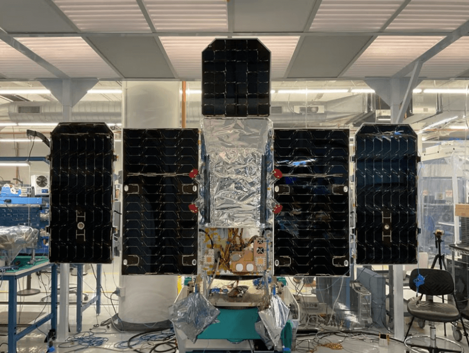
Below is an image of Tanager-1 published by Planet Labs prior to its launch.
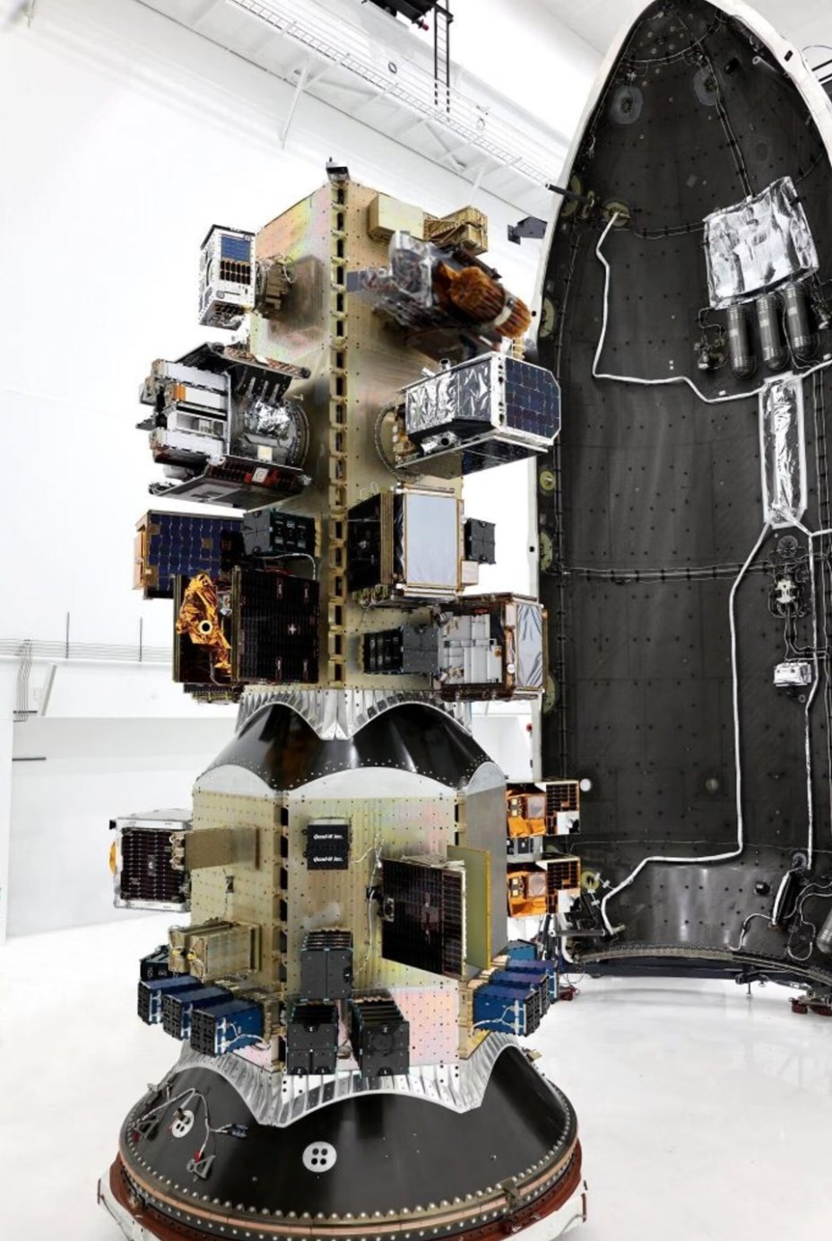
Below is an image SpaceX published of Tanager-1, along with 115 other payloads being readied for launch.
Below is the moment SpaceX deployed Tanager-1 into low earth orbit.
Planet Labs operate an Ephemerides service which gives live status and trajectory information for the satellites in their constellations.
Below is the operation status of Tanager-1 at the time of writing.
$ curl -sL http://ephemerides.planet-labs.com/operational_status.txt \
    | grep -i tanager
The following lists Tanager-1's hardware ID, name, NORAD ID and current status.
4001 Tanager-4001 60507 Operational
Below is Tanager-1's trajectory information at the time of writing, expressed as a two-line element set.
$ curl -s https://ephemerides.planet-labs.com/planet_mc.tle \
    | grep -A2 TANAGER
0 TANAGER 4001 4001
1 60507U PLANET   25204.11440972  .00000000  00000+0  34603-3 0    00
2 60507 097.4024 288.9070 0009426 241.7275 267.6297 15.43677241    08
I'll use Skyfield to estimate Tanager-1's current position over the Earth.
$ python3
from skyfield.api import load, wgs84, EarthSatellite


name  = 'TANAGER 4001 4001'
line1 = '1 60507U PLANET   25204.11440972  .00000000  00000+0  34603-3 0    00'
line2 = '2 60507 097.4024 288.9070 0009426 241.7275 267.6297 15.43677241    08'

ts        = load.timescale()
satellite = EarthSatellite(line1, line2, name, ts)
lat, lon  = wgs84.latlon_of(satellite.at(ts.now()))
print(lon.degrees, lat.degrees)
When I ran the above it reported Tanager-1's position as 72.577, -26.391 which lined up with what n2yo estimated.
Open Data Feed
I'll collect a list of Tanager imagery available from Planet Labs' STAC service. I'll use Mapbox to get the address details of each image as well.
$ mkdir -p ~/hyper
$ cd ~/hyper

$ python3
import json

import geocoder
from   pystac           import Catalog
from   rich.progress    import track
from   shapely.geometry import shape


mapbox_key = '...' # WIP: Replace with your key

root = Catalog.from_file(href='https://www.planet.com/data/stac/tanager-core-imagery/catalog.json')

try:
    recs = [json.loads(l)
            for l in open('enriched.json', 'r').readlines()]
except FileNotFoundError:
    recs = []

seen = set()
found_new = False

for item in track(list(root.get_items(recursive=True))):
    if item.assets['basic_radiance_hdf5'].href in seen:
        continue

    if any([True for x in recs if x['id'] == item.id]):
        continue

    seen.add(item.assets['basic_radiance_hdf5'].href)

    centroid_ = shape(item.geometry).centroid
    resp = geocoder.mapbox([centroid_.y, centroid_.x],
                           key=mapbox_key,
                           method='reverse')

    found_new = True
    recs.append({
        'properties':          item.properties,
        'geom':                shape(item.geometry).wkt,
        'id':                  item.id,
        'bbox':                item.bbox,
        'basic_radiance_hdf5': item.assets['basic_radiance_hdf5'].href,
        'thumbnail':           item.assets['thumbnail'].href,
        'mapbox':              resp.current_result.__dict__ if resp.ok else {},
        'collection_id':       item.collection_id})

if found_new:
    with open('enriched.json', 'w') as f:
        for rec in recs:
            f.write(json.dumps(rec, sort_keys=True) + '\n')
The above produced a 52-line JSONL file. Below is an example record.
$ head -n1 enriched.json | jq -S .
{
  "basic_radiance_hdf5": "https://storage.googleapis.com/open-cogs/planet-stac/release1-basic-radiance/20250511_074311_00_4001_basic_radiance.h5",
  "bbox": [
    53.632003821175445,
    23.990194665823015,
    53.89426128660131,
    24.19200197892316
  ],
  "collection_id": "coastal-water-bodies",
  "geom": "POLYGON ((53.67273222436389 24.19200197892316, 53.632003821175445 24.013441053575885, 53.856983165437306 23.990194665823015, 53.89426128660131 24.16789764336515, 53.67273222436389 24.19200197892316))",
  "id": "20250511_074311_00_4001",
  "mapbox": {
    "_geometry": {
      "coordinates": [
        54.377401,
        24.453835
      ],
      "type": "Point"
    },
    "east": 56.014935,
    "eastnorth": [
      56.014935,
      25.247884
    ],
    "fieldnames": [
      "accuracy",
      "address",
      "bbox",
      "city",
      "confidence",
      "country",
      "housenumber",
      "lat",
      "lng",
      "ok",
      "postal",
      "quality",
      "raw",
      "state",
      "status",
      "street"
    ],
    "json": {
      "address": "Abu Dhabi, United Arab Emirates",
      "bbox": {
        "northeast": [
          25.247884,
          56.014935
        ],
        "southwest": [
          22.631514,
          51.42123
        ]
      },
      "confidence": 1,
      "country": "United Arab Emirates",
      "lat": 24.453835,
      "lng": 54.377401,
      "ok": true,
      "quality": 1,
      "raw": {
        "bbox": [
          51.42123,
          22.631514,
          56.014935,
          25.247884
        ],
        "center": [
          54.377401,
          24.453835
        ],
        "context": [
          {
            "id": "country.8707",
            "mapbox_id": "dXJuOm1ieHBsYzpJZ00",
            "short_code": "ae",
            "text": "United Arab Emirates",
            "wikidata": "Q878"
          }
        ],
        "country": "United Arab Emirates",
        "geometry": {
          "coordinates": [
            54.377401,
            24.453835
          ],
          "type": "Point"
        },
        "id": "region.33795",
        "place_name": "Abu Dhabi, United Arab Emirates",
        "place_type": [
          "region"
        ],
        "properties": {
          "mapbox_id": "dXJuOm1ieHBsYzpoQU0",
          "short_code": "AE-AZ",
          "wikidata": "Q187712"
        },
        "relevance": 1,
        "text": "Abu Dhabi",
        "type": "Feature"
      },
      "status": "OK"
    },
    "north": 25.247884,
    "northeast": [
      25.247884,
      56.014935
    ],
    "northwest": [
      25.247884,
      51.42123
    ],
    "raw": {
      "bbox": [
        51.42123,
        22.631514,
        56.014935,
        25.247884
      ],
      "center": [
        54.377401,
        24.453835
      ],
      "context": [
        {
          "id": "country.8707",
          "mapbox_id": "dXJuOm1ieHBsYzpJZ00",
          "short_code": "ae",
          "text": "United Arab Emirates",
          "wikidata": "Q878"
        }
      ],
      "country": "United Arab Emirates",
      "geometry": {
        "coordinates": [
          54.377401,
          24.453835
        ],
        "type": "Point"
      },
      "id": "region.33795",
      "place_name": "Abu Dhabi, United Arab Emirates",
      "place_type": [
        "region"
      ],
      "properties": {
        "mapbox_id": "dXJuOm1ieHBsYzpoQU0",
        "short_code": "AE-AZ",
        "wikidata": "Q187712"
      },
      "relevance": 1,
      "text": "Abu Dhabi",
      "type": "Feature"
    },
    "south": 22.631514,
    "southeast": [
      22.631514,
      56.014935
    ],
    "southwest": [
      22.631514,
      51.42123
    ],
    "west": 51.42123,
    "westsouth": [
      51.42123,
      22.631514
    ]
  },
  "properties": {
    "constellation": "Tanager",
    "datetime": "2025-05-11T07:43:11Z",
    "description": "Basic (georeferenced, unprojected) core imagery data products from Tanager-1",
    "gsd": 34.77,
    "instruments": [
      "4001"
    ],
    "license": "CC-BY-SA-4.0",
    "platform": "Planet",
    "title": "TanagerScene 20250511_074311_00_4001 Basic Core Imagery",
    "view:azimuth": 209.1,
    "view:off_nadir": 25.8,
    "view:sun_azimuth": 122.8,
    "view:sun_elevation": 79.2
  },
  "thumbnail": "https://storage.googleapis.com/open-cogs/planet-stac/release1-basic-radiance/20250511_074311_00_4001_thumb.png"
}
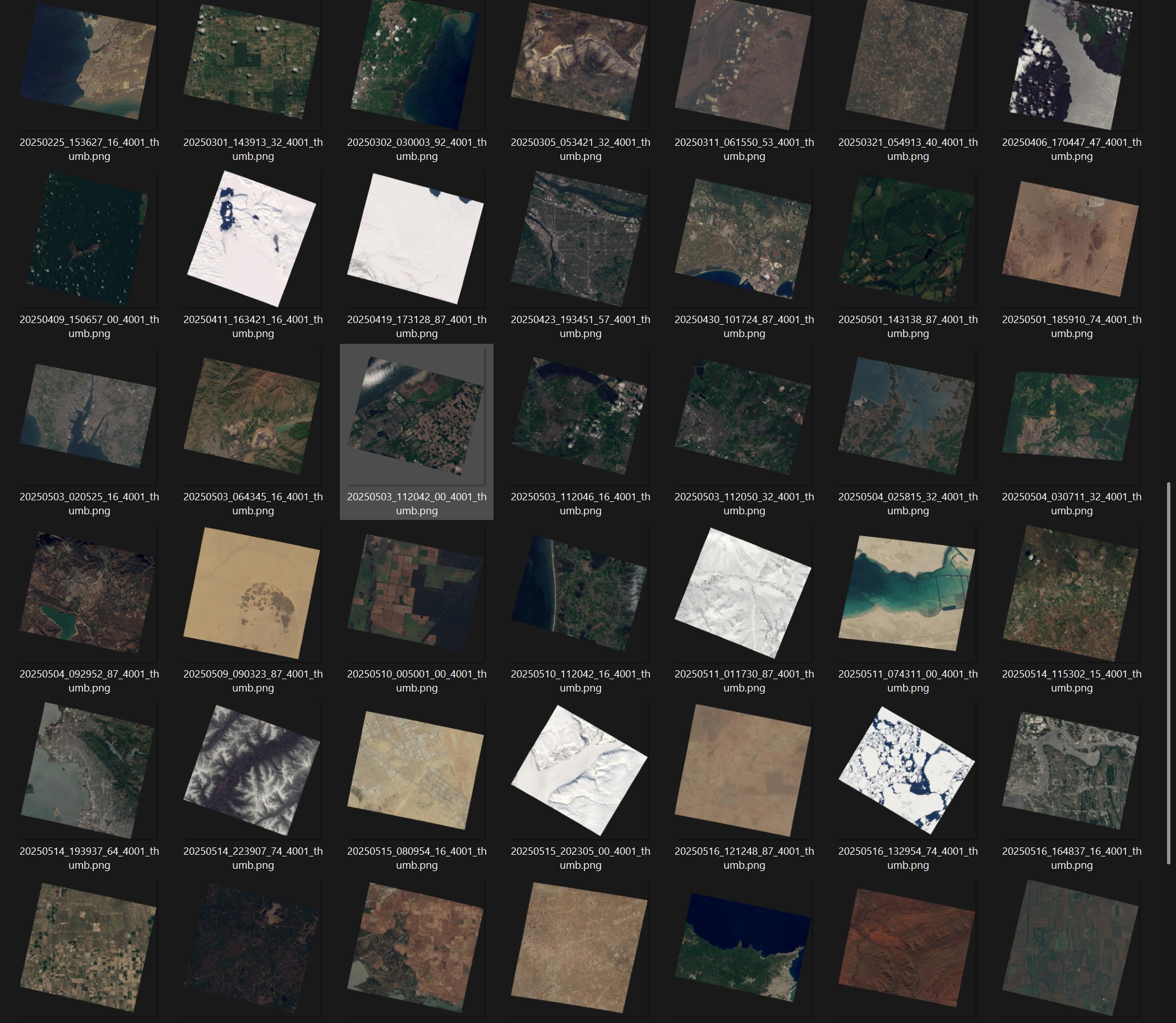
The following will download 37 MB of PNG-formatted thumbnails.
$ jq .thumbnail enriched.json \
    | xargs -P4 \
            -I% \
            wget -qc %
The following will download 25 GB of HDF5-formatted imagery.
$ jq .basic_radiance_hdf5 enriched.json \
    | xargs -P4 \
            -I% \
            wget -qc %
Below is a screenshot of the thumbnails.
I'll generate a Parquet file pin-pointing the location of each image.
$ echo "COPY(
            SELECT id,
                   ST_ASWKB(ST_CENTROID(geom::geometry)) AS geom
            FROM   'enriched.json'
        ) TO 'footprints.parquet' (
            FORMAT            'PARQUET',
            CODEC             'ZSTD',
            COMPRESSION_LEVEL 22,
            ROW_GROUP_SIZE    15000);" \
    | ~/duckdb
The following was rendered in ArcGIS Pro 3.5.
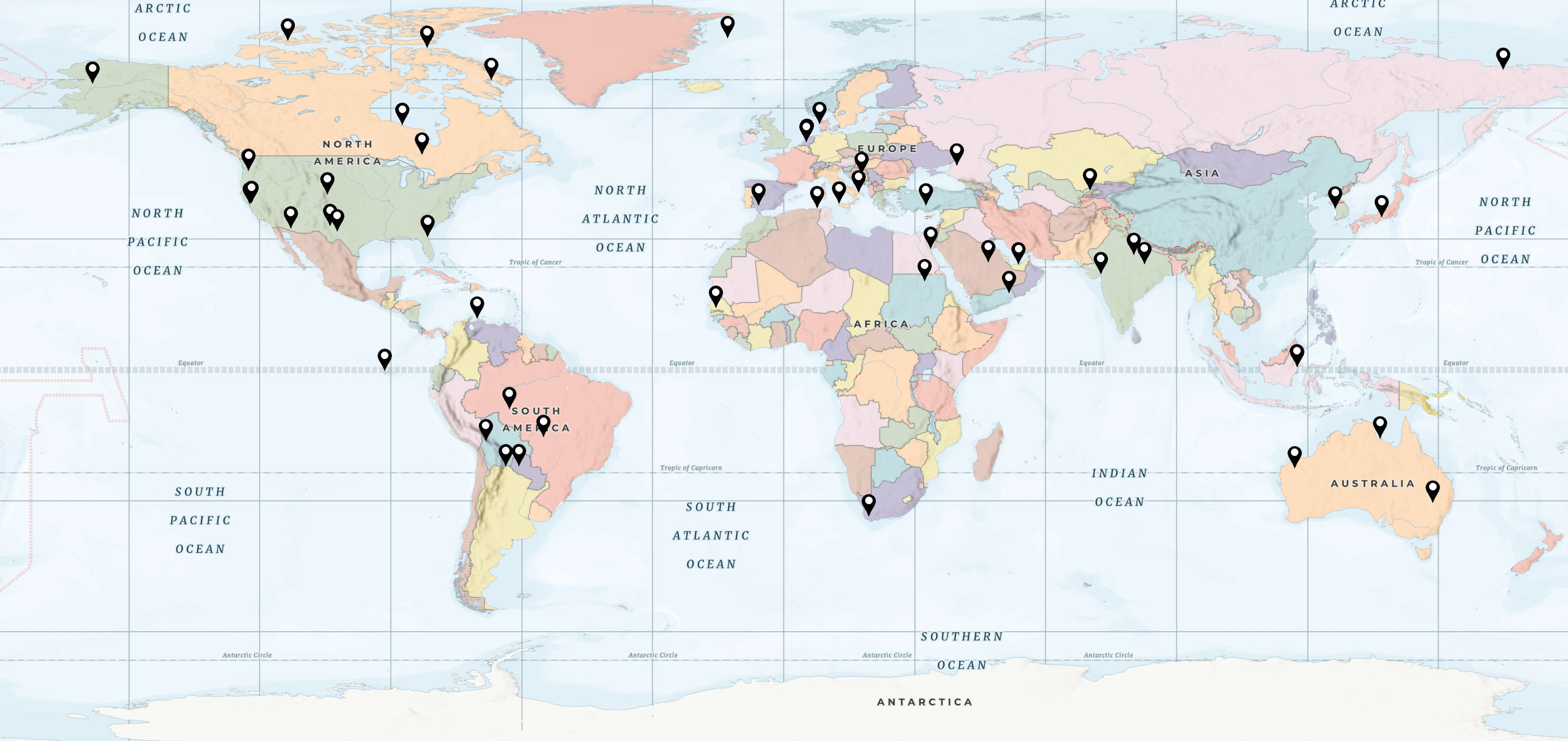
Below I've listed the ID prefix of each image along with the country's footprint it was taken in. The one image missing from this list was taken close to the North Pole.
$ ~/duckdb
.maxrows 100

SELECT   SPLIT(
              SPLIT(basic_radiance_hdf5, '/')[-1],
              '_4001_')[1] AS id_prefix,
         mapbox.json.country
FROM     'enriched.json'
WHERE    mapbox.json.country IS NOT NULL
ORDER BY 2;
┌────────────────────┬────────────────────────┐
│     id_prefix      │        country         │
│      varchar       │        varchar         │
├────────────────────┼────────────────────────┤
│ 20250601_104901_58 │ Algeria                │
│ 20250224_145149_32 │ Argentina              │
│ 20250510_005001_00 │ Australia              │
│ 20250606_030446_90 │ Australia              │
│ 20250608_014315_58 │ Australia              │
│ 20250606_152952_74 │ Bolivia                │
│ 20250221_102048_16 │ Bosnia and Herzegovina │
│ 20250409_150657_00 │ Brazil                 │
│ 20250501_143138_87 │ Brazil                 │
│ 20250419_173128_87 │ Canada                 │
│ 20250520_171055_87 │ Canada                 │
│ 20250515_202305_00 │ Canada                 │
│ 20250606_181248_58 │ Canada                 │
│ 20250411_163421_16 │ Canada                 │
│ 20250510_112042_16 │ Denmark                │
│ 20250406_170447_47 │ Ecuador                │
│ 20250606_090504_75 │ Egypt                  │
│ 20250305_053421_32 │ India                  │
│ 20250311_061550_53 │ India                  │
│ 20250321_054913_40 │ India                  │
│ 20250302_030003_92 │ Indonesia              │
│ 20250504_030711_32 │ Indonesia              │
│ 20250606_103541_58 │ Italy                  │
│ 20250430_101724_87 │ Italy                  │
│ 20250503_020525_16 │ Japan                  │
│ 20250503_112050_32 │ Netherlands            │
│ 20250503_112042_00 │ Netherlands            │
│ 20250503_112046_16 │ Netherlands            │
│ 20250301_143913_32 │ Paraguay               │
│ 20250606_085958_90 │ Russia                 │
│ 20250511_011730_87 │ Russia                 │
│ 20250515_080954_16 │ Saudi Arabia           │
│ 20250516_121248_87 │ Senegal                │
│ 20250504_092952_87 │ South Africa           │
│ 20250504_025815_32 │ South Korea            │
│ 20250514_115302_15 │ Spain                  │
│ 20250509_090323_87 │ Sudan                  │
│ 20250608_091605_90 │ Türkiye                │
│ 20250511_074311_00 │ United Arab Emirates   │
│ 20250516_181930_35 │ United States          │
│ 20250528_180922_74 │ United States          │
│ 20250514_223907_74 │ United States          │
│ 20250521_194038_10 │ United States          │
│ 20250423_193451_57 │ United States          │
│ 20250501_185910_74 │ United States          │
│ 20250205_175845_00 │ United States          │
│ 20250516_164837_16 │ United States          │
│ 20250514_193937_64 │ United States          │
│ 20250503_064345_16 │ Uzbekistan             │
│ 20250225_153627_16 │ Venezuela              │
│ 20250608_074757_58 │ Yemen                  │
├────────────────────┴────────────────────────┤
│ 51 rows                           2 columns │
└─────────────────────────────────────────────┘
Imagery Metadata
Each image contains a large amount of metadata. Below is the non-band and non-STAC metadata for one of their images.
$ gdalinfo -json \
    20250225_153627_16_4001_basic_radiance.tif \
    > 20250225_153627_16_4001_basic_radiance.json
$ jq 'del(.bands)' \
    20250225_153627_16_4001_basic_radiance.json \
    | jq -S 'del(.stac)'
{
  "cornerCoordinates": {
    "center": [
      303.5,
      250.5
    ],
    "lowerLeft": [
      0.0,
      501.0
    ],
    "lowerRight": [
      607.0,
      501.0
    ],
    "upperLeft": [
      0.0,
      0.0
    ],
    "upperRight": [
      607.0,
      0.0
    ]
  },
  "description": "20250225_153627_16_4001_basic_radiance.tif",
  "driverLongName": "GeoTIFF",
  "driverShortName": "GTiff",
  "extent": {
    "coordinates": [
      []
    ],
    "type": "Polygon"
  },
  "files": [
    "20250225_153627_16_4001_basic_radiance.tif"
  ],
  "metadata": {
    "": {
      "HDFEOS_INFORMATION_HDFEOSVersion": "HDFEOS_5.1.15",
      "HDFEOS_SWATHS_HYP_Geolocation_Fields_Planet_Ortho_Framing": "{\"cols\": 778, \"epsg_code\": 32619, \"geotransform\": [355530.0, 30.0, 0.0, 1299210.0, 0.0, -30.0], \"rows\": 657}",
      "HDFEOS_SWATHS_HYP_created_at": "2025-07-12T14:33:39.649432+00:00",
      "HDFEOS_SWATHS_HYP_strip_id": "20250225_153623_00_4001_strip"
    },
    "IMAGE_STRUCTURE": {
      "INTERLEAVE": "PIXEL"
    }
  },
  "size": [
    607,
    501
  ]
}
The metadata documents each of the 426 bands collected in each image.
$ jq '.bands[]|.metadata."".wavelengths' \
    20250225_153627_16_4001_basic_radiance.json \
    | wc -l # 426
Below is the metadata for an individual band within one of their images.
$ jq '.bands[0]' 20250225_153627_16_4001_basic_radiance.json
{
  "band": 1,
  "block": [
    607,
    1
  ],
  "type": "Float32",
  "colorInterpretation": "Gray",
  "metadata": {
    "": {
      "applied_radiometric_coefficient": "0.24117877",
      "applied_radiometric_coefficients_units": "W/(m^2 sr um)",
      "fwhm": "5.3899999",
      "fwhm_units": "nm",
      "Unit": "W/(m^2 sr um)",
      "wavelengths": "376.44",
      "wavelengths_units": "nm"
    }
  }
}
Below are the first 10 wavelengths in one of their images.
$ jq '.bands[]|.metadata."".wavelengths' \
    20250225_153627_16_4001_basic_radiance.json \
    | head
"376.44"
"381.41"
"386.38"
"391.35001"
"396.32001"
"401.29001"
"406.26001"
"411.23001"
"416.20999"
"421.17999"
The GSD appears to be unique for each of the 52 images in this dataset.
$ jq -S .properties.gsd enriched.json | sort
32.58
32.62
32.64
...
38.98
39.1
39.12
According to their documentation, their Tanager-1 imagery goes through the following processing steps before publication.
- Dark Subtraction
- Pedestal Correction
- Flat Field Correction
- Bad Pixel Correction
- Optical Scatter Correction
- Optical Ghost Correction
- Absolute Radiometric Calibration
- Order Sorting Filter (OSF) Seam Correction
- Visual Product Processing
- Orthorectification
- Atmospheric Correction
They state they use ISOFIT in the Atmospheric Correction stage. The two biggest contributors to this project both work at NASA’s Jet Propulsion Laboratory.
QGIS
QGIS can open Planet Labs' HDF5 files as they are but won't georeference them properly. Below you can see each field as its own layer with the toa_radiance field on top. I've adjusted the red, green and blue bands assignments from what QGIS selected by default.
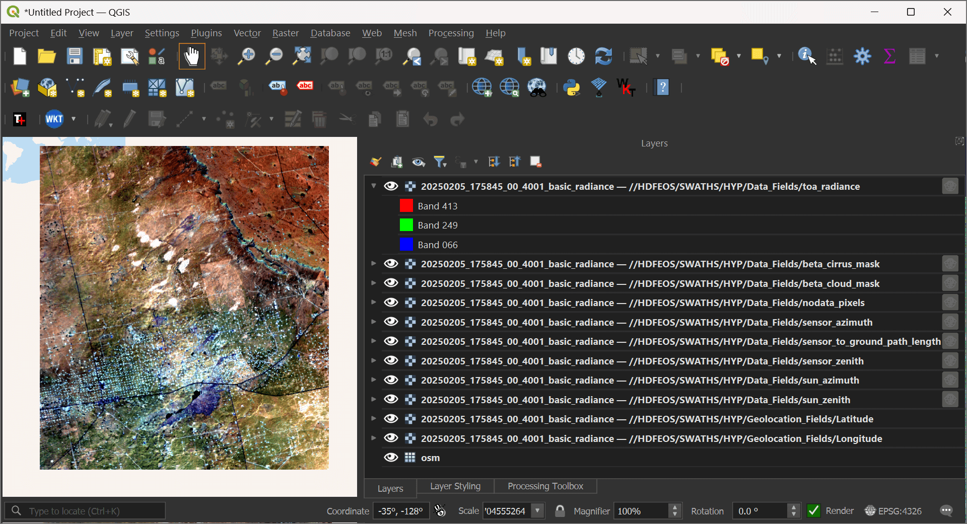
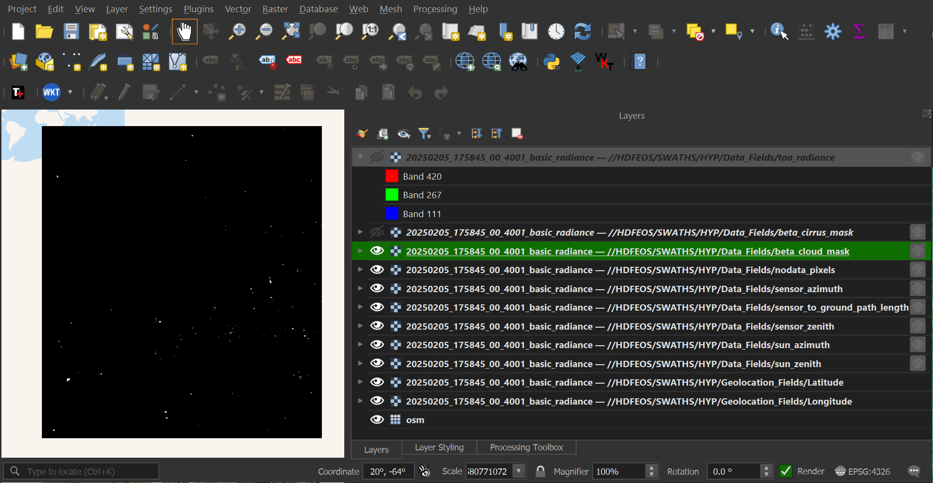
Each image comes with a cloud mask layer as well. This helps exclude cloud-covered areas from any calculations or processing you'd run the image through.
The following will convert an HDF5 file from Planet Labs into a georeferenced GeoTIFF. It will position itself automatically when dropped into a QGIS workbook.
$ gdalwarp \
    -t_srs "EPSG:4326" \
    HDF5:"20250225_153627_16_4001_basic_radiance.h5"://HDFEOS/SWATHS/HYP/Data_Fields/toa_radiance  \
    test.tif
Note, only the toa_radiance data will be copied into the above GeoTIFF. I'll discuss this more later on but I'm working on a script that can make Planet Labs' HDF5s more analysis-ready.
ArcGIS Pro
I tried to import an HDF5 file into ArcGIS Pro 3.5. It sat at the following screen for some time.
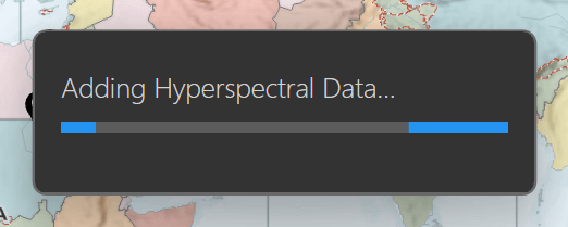
After a while, it began reporting XML below the progress bar.
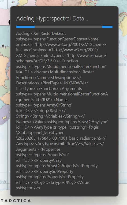
After 30+ minutes, only the beta_cirrus_mask layer was imported.
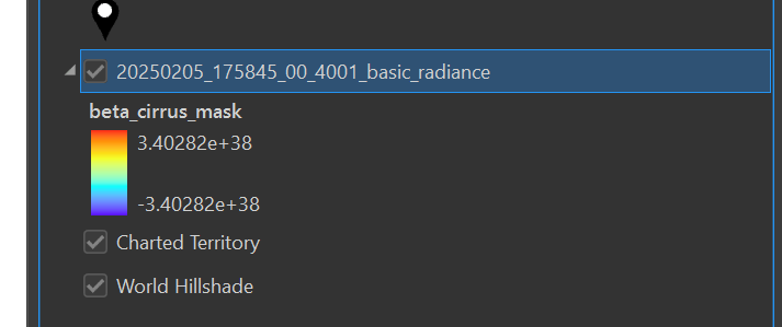
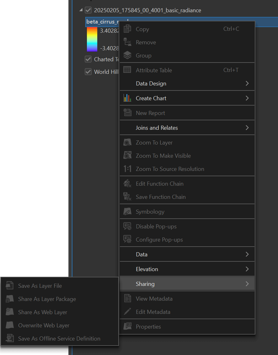
Very few tools were available for this layer.
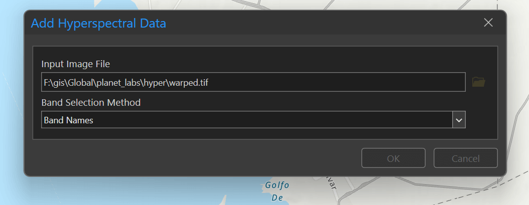
I then tried to import the GeoTIFF I had produced earlier. ArcGIS Pro 3.5 sat here for an hour before I gave up.
I did a review of Wyvern's Hyperspectral Imagery a while back. Their GeoTIFFs can be dropped into ArcGIS Pro 3.5, have ideal RGB bands selected and rendered in under a minute on my machine. Below is one such image.
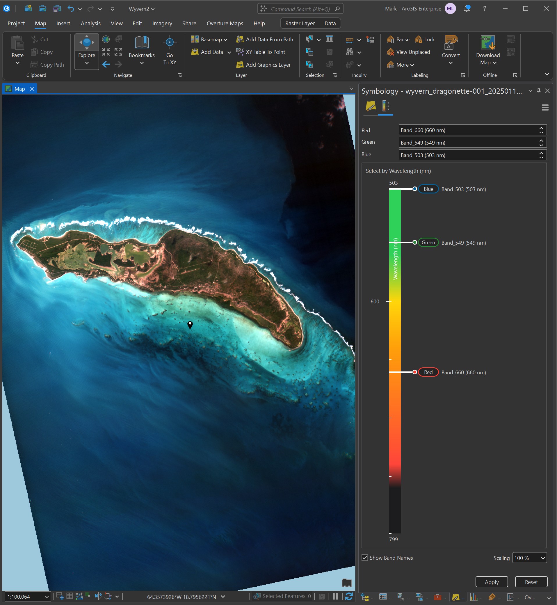
I need to figure out how to convert Planet Labs' HDF5s into this sort of analysis-ready GeoTIFF.
HyperCoast
Over the past year, Qiusheng Wu of the University of Tennessee has been working on HyperCoast, a python package for visualising and analysing hyperspectral imagery.
I'll launch Jupyter Lab from the same folder containing Planet Labs' HDF5 files. Note, I had to run the following from a dedicated Ubuntu Desktop 24 VM as I'm battling a networking issue with WSL.
$ cd ~/hyper

$ jupyter lab \
    --no-browser \
    --ip=0.0.0.0 \
    --NotebookApp.iopub_data_rate_limit=100000000
I'll create a new Python 3 notebook and run the following to render one of Planet Labs' images.
import hypercoast


dataset = hypercoast.read_tanager('20250608_074757_58_4001_basic_radiance.h5')
m = hypercoast.Map()
m.add_tanager(dataset,
              bands=[100, 60, 50],
              vmin=0,
              vmax=120,
              layer_name='Tanager')
m.add('spectral')
m
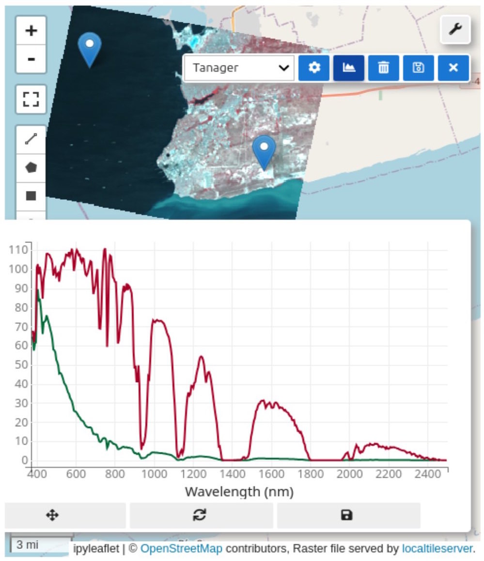
Below I've marked two points on Tanager-1's image of Venezuela. The point on the left is in the sea and its spectral signature is in green. The point on the right has its spectral signature drawn in red.
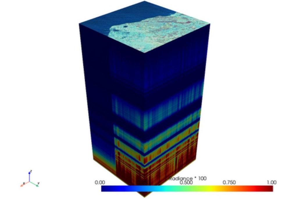
HyperCoast can render hyperspectral imagery as a 3D cube. Below is a cube for the above image of Venezuela.
gridded = hypercoast.grid_tanager(dataset,
                                  row_range=(200, 400),
                                  col_range=(200, 400))
gridded = (gridded / 100).clip(0, 1)

cube = hypercoast.image_cube(
    gridded,
    variable='toa_radiance',
    cmap='jet',
    clim=(0, 1),
    rgb_wavelengths=[1000, 600, 500],
    title='Radiance * 100',
)
cube.show()
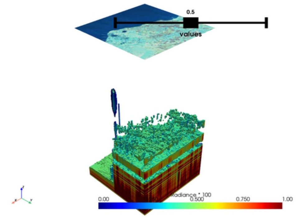
The 3D cubes can also be sliced, including with an interactive threshold, as shown below.
Awesome Spectral Indices
The Awesome Spectral Indices project lists hundreds of chemical and naturally-occurring phenomenon that can be detected from hyperspectral imagery.

The spectral signature analysis above is useful as it can be paired with known algorithms that can identify things in hyperspectral imagery that are either invisible to the naked eye or hard to confirm with RGB imagery alone.
Below are a few of the soil-specific indices listed in the project.
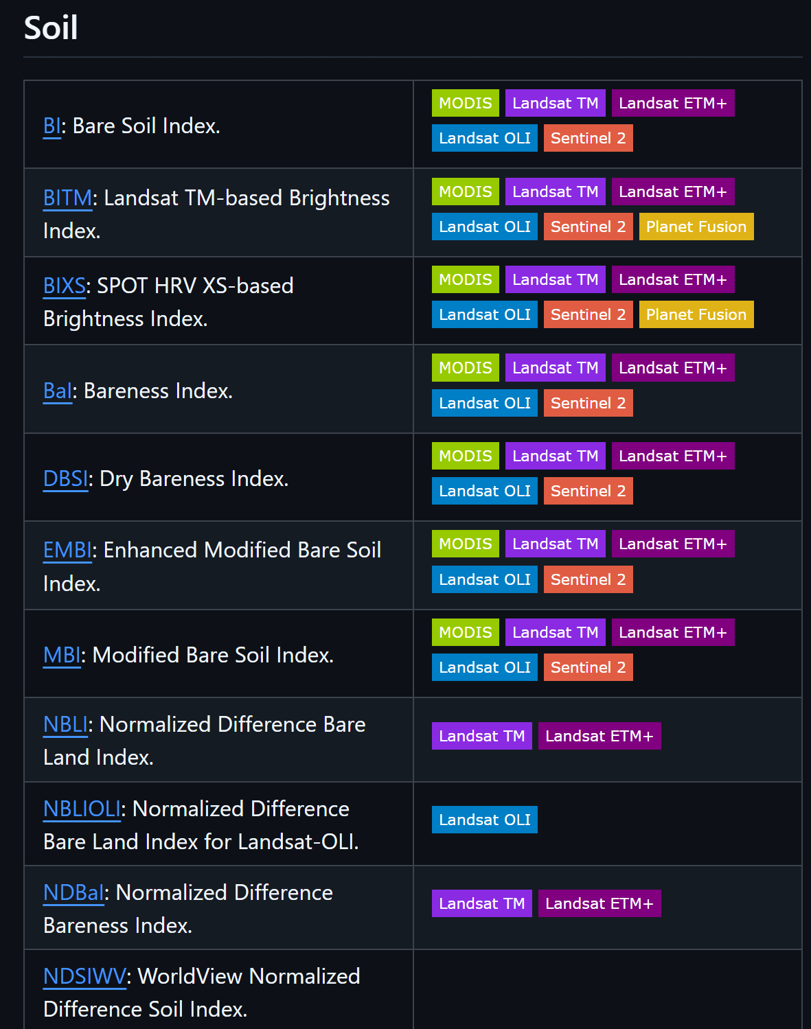
There is a package called spyndex which provides Python bindings for the project as well.