Last month, Wyvern, a 36-person start-up with $16M USD in funding in Edmonton, Canada launched an open data programme for their VNIR, 23 to 31-band hyperspectral satellite imagery.
The imagery was captured with one of their three Dragonette 6U CubeSat satellites. These satellites were built by AAC Clyde Space which has offices in the UK, Sweden and a few other countries. They orbit 517 - 550 KM above the Earth's surface and have a spatial resolution at nadir (GSD) of 5.3M.
SpaceX launched all three of their satellites from Vandenberg Space Force Base in California. They were launched on April 15th, June 12th and November 11th, 2023 respectively.

There are ~130 GB of GeoTIFFs being hosted in their AWS S3 bucket in Montreal. The 33 images posted were taken between June and two weeks ago.
In this post, I'll examine Wyvern's open data feed.
My Workstation
I'm using a 5.7 GHz AMD Ryzen 9 9950X CPU. It has 16 cores and 32 threads and 1.2 MB of L1, 16 MB of L2 and 64 MB of L3 cache. It has a liquid cooler attached and is housed in a spacious, full-sized Cooler Master HAF 700 computer case.
The system has 96 GB of DDR5 RAM clocked at 4,800 MT/s and a 5th-generation, Crucial T700 4 TB NVMe M.2 SSD which can read at speeds up to 12,400 MB/s. There is a heatsink on the SSD to help keep its temperature down. This is my system's C drive.
The system is powered by a 1,200-watt, fully modular Corsair Power Supply and is sat on an ASRock X870E Nova 90 Motherboard.
I'm running Ubuntu 24 LTS via Microsoft's Ubuntu for Windows on Windows 11 Pro. In case you're wondering why I don't run a Linux-based desktop as my primary work environment, I'm still using an Nvidia GTX 1080 GPU which has better driver support on Windows and I use ArcGIS Pro from time to time which only supports Windows natively.
Installing Prerequisites
I'll use GDAL 3.9.3, Python 3.12.3 and a few other tools to help analyse the data in this post.
$ sudo add-apt-repository ppa:deadsnakes/ppa
$ sudo add-apt-repository ppa:ubuntugis/ubuntugis-unstable
$ sudo apt update
$ sudo apt install \
    gdal-bin \
    jq \
    libimage-exiftool-perl \
    libtiff-tools \
    python3-pip \
    python3.12-venv
I'll set up a Python Virtual Environment and install some dependencies.
$ python3 -m venv ~/.wyvern
$ source ~/.wyvern/bin/activate
$ python3 -m pip install \
    astropy \
    geocoder \
    pystac \
    rich \
    shapely \
    sgp4
I'll use my GeoTIFFs analysis utility in this post.
$ git clone https://github.com/marklit/geotiffs \
    ~/geotiffs
$ python3 -m pip install \
          -r ~/geotiffs/requirements.txt
I'll use DuckDB, along with its H3, JSON, Lindel, Parquet and Spatial extensions, in this post.
$ cd ~
$ wget -c https://github.com/duckdb/duckdb/releases/download/v1.1.3/duckdb_cli-linux-amd64.zip
$ unzip -j duckdb_cli-linux-amd64.zip
$ chmod +x duckdb
$ ~/duckdb
INSTALL h3 FROM community;
INSTALL lindel FROM community;
INSTALL json;
INSTALL parquet;
INSTALL spatial;
I'll set up DuckDB to load every installed extension each time it launches.
$ vi ~/.duckdbrc
.timer on
.width 180
LOAD h3;
LOAD lindel;
LOAD json;
LOAD parquet;
LOAD spatial;
The maps in this post were rendered with QGIS version 3.42. QGIS is a desktop application that runs on Windows, macOS and Linux. The application has grown in popularity in recent years and has ~15M application launches from users all around the world each month.
I used QGIS' Tile+ plugin to add geospatial context with Bing's Virtual Earth Basemap as well as CARTO's to the maps. The dark, non-satellite imagery maps are mostly made up of vector data from Natural Earth and Overture.
Dragonette's Satellites
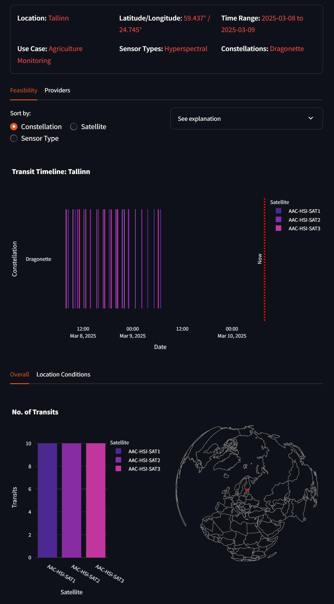
Below is PulseOrbital's list of estimated Tallinn flyovers by Wyvern's Dragonette constellation for March 8th and 9th, 2025.
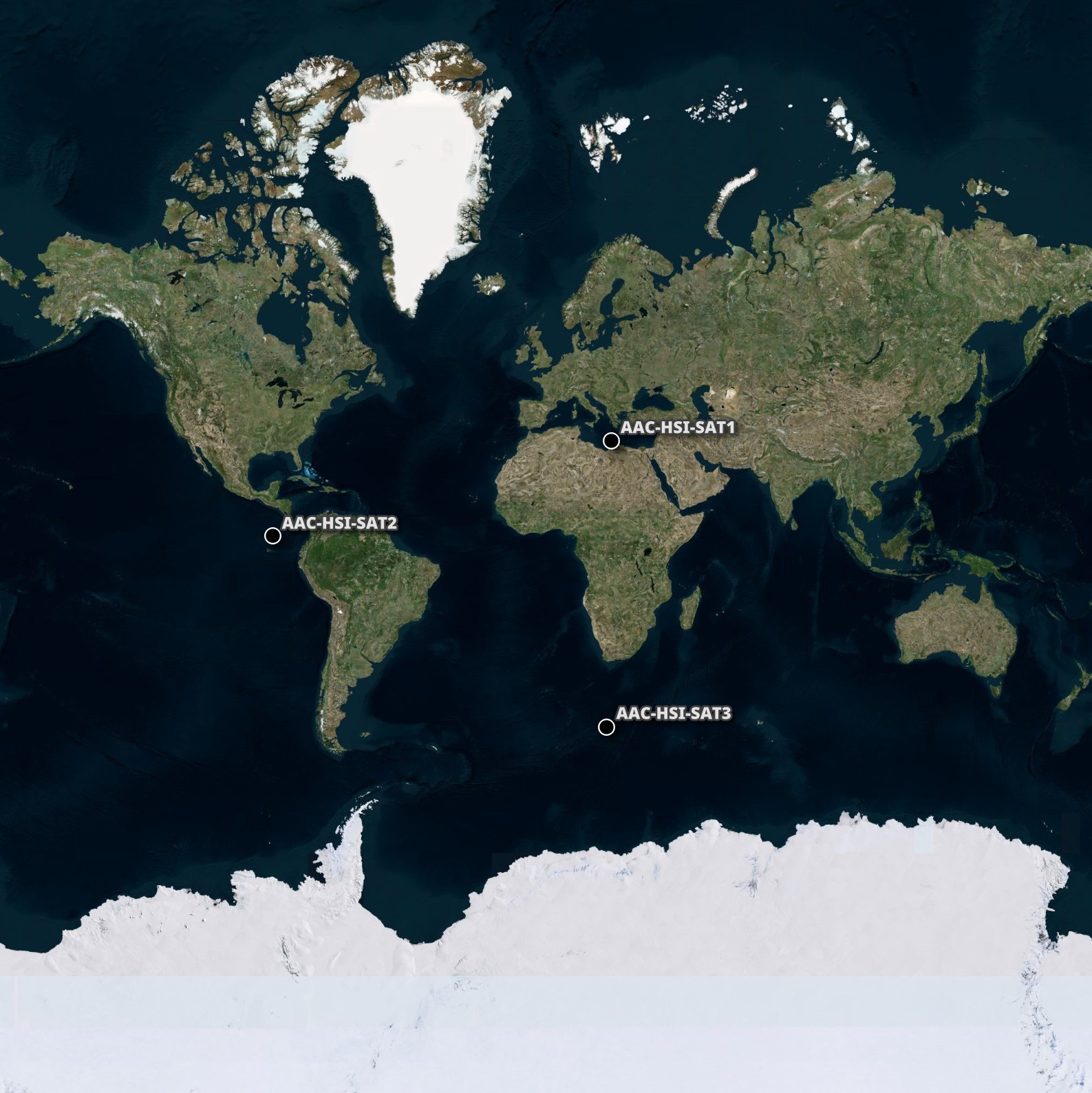
Below I'll try to estimate the current locations of each of their three satellites. I found the Two-line elements (TLE) details on n2yo.
I ran the following on March 10th, 2025. It produced a CSV file with names and estimated locations of their three satellites.
$ python3
from   datetime            import datetime, UTC
import json

from   astropy             import units as u
from   astropy.time        import Time
from   astropy.coordinates import ITRS, \
                                  TEME, \
                                  CartesianDifferential, \
                                  CartesianRepresentation
from   sgp4.api            import Satrec
from   sgp4.api            import SGP4_ERRORS


tles = '''AAC-HSI-SAT1
          1 56225U 23054AZ  25068.93354999  .00004447  00000-0  28073-3 0  9998
          2 56225  97.4339 315.2974 0008749 291.1678  68.8616 15.09548670105253
          AAC-HSI-SAT2
          1 56995U 23084BX  25069.13857882  .00006243  00000-0  33207-3 0  9998
          2 56995  97.7590 200.5235 0013312 352.0602   8.0417 15.15565025 95939
          AAC-HSI-SAT3
          1 58848U 23174DH  25068.89805865  .00005229  00000-0  30564-3 0  9999
          2 58848  97.4007 137.8776 0011809 171.1785 188.9655 15.12246107 73641
          '''.strip().splitlines()

with open('locations.csv', 'w') as f:
    while tles:
        name  = tles.pop(0).strip()
        line1 = tles.pop(0).strip()
        line2 = tles.pop(0).strip()

        satellite = Satrec.twoline2rv(line1, line2)

        t = Time(datetime.now(UTC).isoformat().split('+')[0],
                 format='isot',
                 scale='utc')

        error_code, teme_p, teme_v = satellite.sgp4(t.jd1, t.jd2) # in km and km/s

        if error_code != 0:
            raise RuntimeError(SGP4_ERRORS[error_code])

        teme_p = CartesianRepresentation(teme_p * u.km)
        teme_v = CartesianDifferential(teme_v * u.km / u.s)
        teme = TEME(teme_p.with_differentials(teme_v), obstime=t)

        itrs_geo = teme.transform_to(ITRS(obstime=t))
        location = itrs_geo.earth_location
        loc = location.geodetic

        f.write('"%s", "POINT (%f %f)"\n' % (name,
                                             loc.lon.deg,
                                             loc.lat.deg))
Below is a rendering of the above CSV data in QGIS.
Open Data Feed
Wyvern have a STAC catalog listing the imagery locations and metadata around their capture. I'll download this metadata and get each image's address details with Mapbox's reverse geocoding service. Mapbox offer 100K geocoding searches per month with their free tier.
$ python3
import json

import geocoder
from   pystac           import Catalog
from   rich.progress    import track
from   shapely.geometry import shape


mapbox_key = '...' # WIP: Replace with your key
root = Catalog.from_file(href='https://wyvern-prod-public-open-data-program.s3.ca-central-1.amazonaws.com/catalog.json')

seen = set()

with open('enriched.json', 'w') as f:
    for item in track(list(root.get_items(recursive=True))):
        if item.assets['Cloud optimized GeoTiff'].href in seen:
            continue

        seen.add(item.assets['Cloud optimized GeoTiff'].href)
        centroid_ = shape(item.geometry).centroid
        resp = geocoder.mapbox([centroid_.y, centroid_.x],
                               key=mapbox_key,
                               method='reverse')
        assert resp.ok is True, resp.status

        f.write(json.dumps(
            {'properties':    item.properties,
             'geom':          shape(item.geometry).wkt,
             'id':            item.id,
             'bbox':          item.bbox,
             'assets':        {k.lower().replace(' ', '_'): v.href
                               for k, v in item.assets.items()},
             'mapbox':        resp.current_result.__dict__,
             'collection_id': item.collection_id},
            sort_keys=True) + '\n')
The above produced a 33-line JSONL file. Below is an example record.
$ head -n1 enriched.json | jq -S .
{
  "assets": {
    "cloud_optimized_geotiff": "https://wyvern-prod-public-open-data-program.s3.ca-central-1.amazonaws.com/wyvern_dragonette-001_20240703T171837_4c406dd3/wyvern_dragonette-001_20240703T171837_4c406dd3.tiff",
    "data_mask": "https://wyvern-prod-public-open-data-program.s3.ca-central-1.amazonaws.com/wyvern_dragonette-001_20240703T171837_4c406dd3/wyvern_dragonette-001_20240703T171837_4c406dd3_data_mask.tiff",
    "overview_image": "https://wyvern-prod-public-open-data-program.s3.ca-central-1.amazonaws.com/wyvern_dragonette-001_20240703T171837_4c406dd3/wyvern_dragonette-001_20240703T171837_4c406dd3_preview.png",
    "pixel_quality_mask": "https://wyvern-prod-public-open-data-program.s3.ca-central-1.amazonaws.com/wyvern_dragonette-001_20240703T171837_4c406dd3/wyvern_dragonette-001_20240703T171837_4c406dd3_pixel_quality_mask.tiff",
    "thumbnail_image": "https://wyvern-prod-public-open-data-program.s3.ca-central-1.amazonaws.com/wyvern_dragonette-001_20240703T171837_4c406dd3/wyvern_dragonette-001_20240703T171837_4c406dd3_thumbnail.png"
  },
  "bbox": [
    -117.14246656709959,
    48.26920917388883,
    -116.64844506075083,
    48.6222705607206
  ],
  "collection_id": "2024",
  "geom": "POLYGON ((-117.09090885825756 48.570741224333794, -117.09090885825756 48.57083115336763, -117.09070614118478 48.570876117884545, -117.08948983874814 48.57110094046913, -117.08847625338427 48.5712807985368, -117.07421848593255 48.57370888245031, -117.04800041118719 48.57816036962509, -117.03975658356107 48.57955426964951, -117.02671511854598 48.58175753097844, -117.01522781775549 48.58369100520587, -117.00319993810427 48.58571440846713, -116.98792858528867 48.5882773859314, -116.96988676581184 48.59129000856483, -116.9558317154329 48.593628163444514, -116.9458310065094 48.59529185057044, -116.93900619839269 48.596415963493364, -116.89765191554693 48.60320560554782, -116.89461115945532 48.60370021523391, -116.8650144668304 48.60851141854402, -116.85089184409387 48.61080460890678, -116.84812137743262 48.61125425407595, -116.84589148963212 48.61161397021129, -116.81298375148523 48.616919783207486, -116.81237560026692 48.616919783207486, -116.81217288319415 48.6164251735214, -116.81183502140618 48.61552588318306, -116.81122687018787 48.61390716057405, -116.80784825230832 48.60486929267375, -116.78994157754666 48.556667330538794, -116.77967057919281 48.52901415263488, -116.77095374506355 48.50554267480424, -116.76811570604472 48.49789870692836, -116.70905746551009 48.33845452994091, -116.70371924926037 48.324020920010575, -116.7027732362541 48.32145794254631, -116.70250294682374 48.32069354575872, -116.70250294682374 48.32042375865722, -116.70257051918134 48.320378794140304, -116.7035841045452 48.320198936072636, -116.70412468340592 48.3201090070388, -116.97833331051073 48.275054561088034, -116.98002261945051 48.27478477398653, -116.9801577641657 48.27478477398653, -116.98022533652329 48.27482973850345, -116.98036048123846 48.275054561088034, -116.98049562595365 48.27541427722337, -116.98069834302642 48.27595385142637, -116.99819958364253 48.32267198450307, -117.03381021609304 48.417906831333134, -117.0373239786878 48.42730441536877, -117.0754347883692 48.529238975219464, -117.07881340624874 48.53827684311977, -117.08861139809946 48.56449115648234, -117.09003041760887 48.56831314042028, -117.09084128589997 48.57051640174921, -117.09090885825756 48.570741224333794))",
  "id": "wyvern_dragonette-001_20240703T171837_4c406dd3",
  "mapbox": {
    "_geometry": {
      "coordinates": [
        -116.89724,
        48.44575
      ],
      "type": "Point"
    },
    "fieldnames": [
      "accuracy",
      "address",
      "bbox",
      "city",
      "confidence",
      "country",
      "housenumber",
      "lat",
      "lng",
      "ok",
      "postal",
      "quality",
      "raw",
      "state",
      "status",
      "street"
    ],
    "json": {
      "address": "38 Miller Gulch, Priest River, Idaho 83821, United States",
      "city": "Priest River",
      "country": "United States",
      "housenumber": "38",
      "lat": 48.44575,
      "lng": -116.89724,
      "ok": true,
      "postal": "83821",
      "quality": 1,
      "raw": {
        "address": "38",
        "center": [
          -116.89724,
          48.44575
        ],
        "context": [
          {
            "id": "postcode.8128753314501880",
            "text": "83821"
          },
          {
            "id": "place.268052716",
            "mapbox_id": "dXJuOm1ieHBsYzpEL29vN0E",
            "text": "Priest River",
            "wikidata": "Q1517705"
          },
          {
            "id": "district.1885932",
            "mapbox_id": "dXJuOm1ieHBsYzpITWJz",
            "text": "Bonner County",
            "wikidata": "Q483932"
          },
          {
            "id": "region.58604",
            "mapbox_id": "dXJuOm1ieHBsYzo1T3c",
            "short_code": "US-ID",
            "text": "Idaho",
            "wikidata": "Q1221"
          },
          {
            "id": "country.8940",
            "mapbox_id": "dXJuOm1ieHBsYzpJdXc",
            "short_code": "us",
            "text": "United States",
            "wikidata": "Q30"
          }
        ],
        "country": "United States",
        "district": "Bonner County",
        "geometry": {
          "coordinates": [
            -116.89724,
            48.44575
          ],
          "type": "Point"
        },
        "id": "address.8128753314501880",
        "place": "Priest River",
        "place_name": "38 Miller Gulch, Priest River, Idaho 83821, United States",
        "place_type": [
          "address"
        ],
        "postcode": "83821",
        "properties": {
          "accuracy": "point",
          "mapbox_id": "dXJuOm1ieGFkcjplYWRmMWVhNi03MDg3LTQzNjUtOWNkNi05NGFjMWNlZTA5NDg"
        },
        "region": "Idaho",
        "relevance": 1,
        "text": "Miller Gulch",
        "type": "Feature"
      },
      "state": "Idaho",
      "status": "OK"
    },
    "northeast": [],
    "northwest": [],
    "raw": {
      "address": "38",
      "center": [
        -116.89724,
        48.44575
      ],
      "context": [
        {
          "id": "postcode.8128753314501880",
          "text": "83821"
        },
        {
          "id": "place.268052716",
          "mapbox_id": "dXJuOm1ieHBsYzpEL29vN0E",
          "text": "Priest River",
          "wikidata": "Q1517705"
        },
        {
          "id": "district.1885932",
          "mapbox_id": "dXJuOm1ieHBsYzpITWJz",
          "text": "Bonner County",
          "wikidata": "Q483932"
        },
        {
          "id": "region.58604",
          "mapbox_id": "dXJuOm1ieHBsYzo1T3c",
          "short_code": "US-ID",
          "text": "Idaho",
          "wikidata": "Q1221"
        },
        {
          "id": "country.8940",
          "mapbox_id": "dXJuOm1ieHBsYzpJdXc",
          "short_code": "us",
          "text": "United States",
          "wikidata": "Q30"
        }
      ],
      "country": "United States",
      "district": "Bonner County",
      "geometry": {
        "coordinates": [
          -116.89724,
          48.44575
        ],
        "type": "Point"
      },
      "id": "address.8128753314501880",
      "place": "Priest River",
      "place_name": "38 Miller Gulch, Priest River, Idaho 83821, United States",
      "place_type": [
        "address"
      ],
      "postcode": "83821",
      "properties": {
        "accuracy": "point",
        "mapbox_id": "dXJuOm1ieGFkcjplYWRmMWVhNi03MDg3LTQzNjUtOWNkNi05NGFjMWNlZTA5NDg"
      },
      "region": "Idaho",
      "relevance": 1,
      "text": "Miller Gulch",
      "type": "Feature"
    },
    "southeast": [],
    "southwest": []
  },
  "properties": {
    "constellation": "Dragonette",
    "created": "2024-11-01T23:03:41Z",
    "datetime": "2024-07-03T17:18:40.010328Z",
    "end_datetime": "2024-07-03T17:18:42.438451Z",
    "eo:cloud_cover": 5.63,
    "gsd": 5.26,
    "instruments": [
      "VNIR Hyperspectral Imaging Sensor"
    ],
    "license": "other",
    "platform": "Dragonette-001",
    "processing:facility": "Wyvern",
    "processing:level": "L1B",
    "processing:version": "1.3",
    "product_type": "hyperspectral",
    "proj:code": "EPSG:4326",
    "proj:shape": [
      7311,
      7852
    ],
    "providers": [
      {
        "name": "Wyvern Inc.",
        "roles": [
          "licensor",
          "producer",
          "processor"
        ],
        "url": "https://www.wyvern.space/"
      }
    ],
    "sat:platform_international_designator": "2023-054AZ",
    "sensor_mode": "strip",
    "sensor_type": "optical",
    "start_datetime": "2024-07-03T17:18:37.582204Z",
    "updated": "2024-11-01T23:03:41Z",
    "view:azimuth": 65.36472836367665,
    "view:incidence_angle": 2.106011989129783,
    "view:off_nadir": 2.6882806109241932,
    "view:sun_azimuth": 116.34019361959561,
    "view:sun_elevation": 50.52691114712514,
    "wyvern:radiometric_resolution": "12"
  }
}
Data Fluency
I'll load their imagery metadata into DuckDB for analysis.
$ ~/duckdb wyvern.duckdb
CREATE OR REPLACE TABLE imagery AS
    FROM READ_JSON('enriched.json');
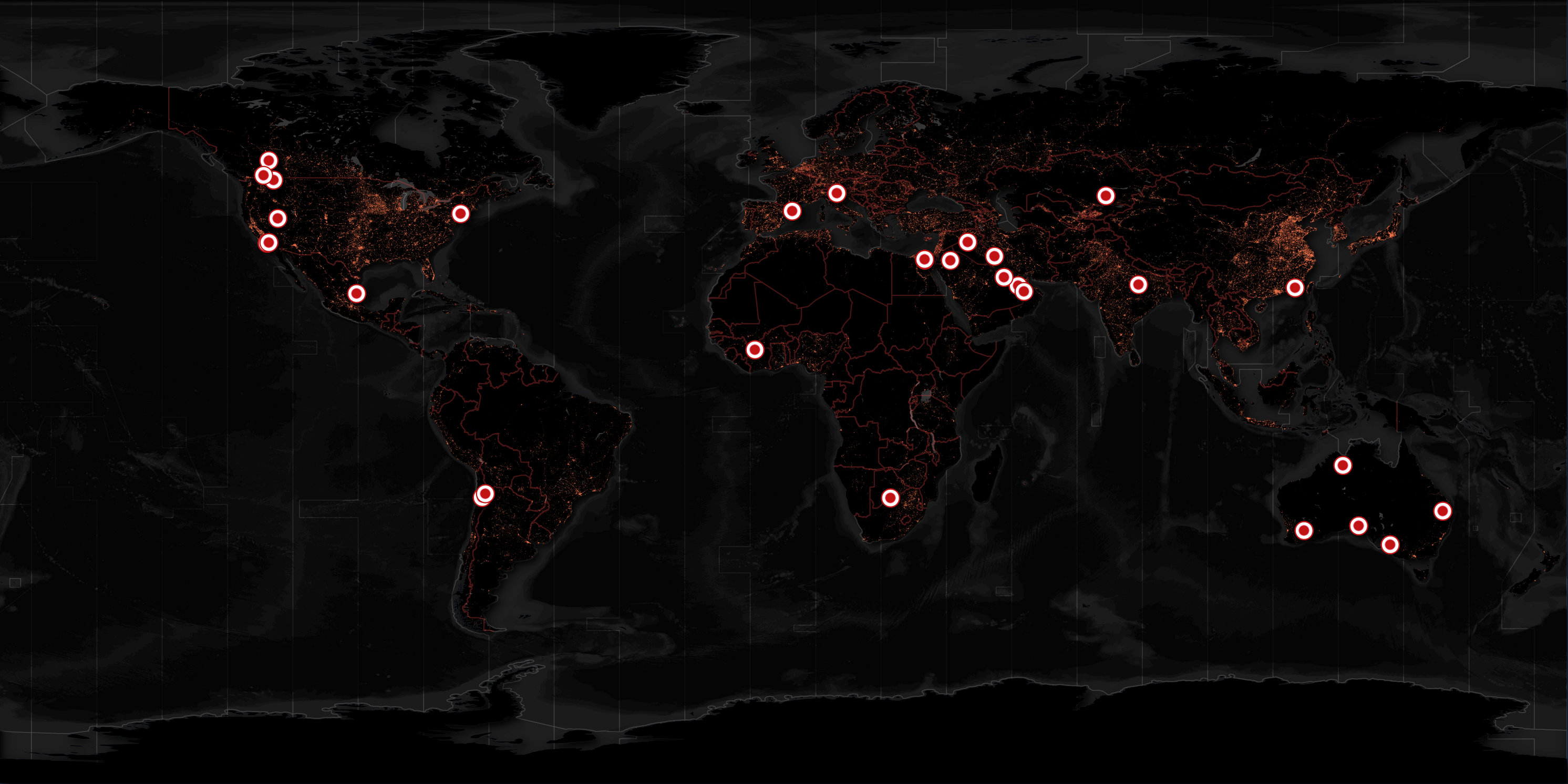
Below are the image counts by country and city. Some areas are rural and Mapbox didn't attribute any city to the image footprint's location.
SELECT   COUNT(*),
         mapbox.json.country,
         mapbox.json.city
FROM     imagery
GROUP BY 2, 3
ORDER BY 2, 3;
┌──────────────┬──────────────────────┬──────────────────────┐
│ count_star() │       country        │         city         │
│    int64     │       varchar        │       varchar        │
├──────────────┼──────────────────────┼──────────────────────┤
│            1 │ Australia            │ Jervois              │
│            1 │ Australia            │ Norwin               │
│            1 │ Australia            │ Ord River            │
│            1 │ Australia            │ Skeleton Rock        │
│            1 │ Australia            │ Yellabinna           │
│            1 │ Bahrain              │                      │
│            1 │ Botswana             │                      │
│            1 │ Canada               │ Beaverdell           │
│            1 │ Canada               │ Jasper               │
│            1 │ Chile                │ Antofagasta          │
│            1 │ Chile                │ San Pedro de Atacama │
│            1 │ China                │                      │
│            1 │ Côte d'Ivoire        │                      │
│            2 │ Egypt                │ Al Ganaeen           │
│            2 │ Egypt                │ Al Qantara East      │
│            1 │ India                │ Gurh                 │
│            1 │ Iran                 │                      │
│            1 │ Iraq                 │                      │
│            1 │ Italy                │                      │
│            1 │ Kazakhstan           │                      │
│            1 │ Mexico               │ Altamira             │
│            1 │ Oman                 │                      │
│            1 │ Saudi Arabia         │                      │
│            1 │ Spain                │ Barcelona            │
│            1 │ United Arab Emirates │                      │
│            1 │ United States        │ Eureka               │
│            2 │ United States        │ Los Angeles          │
│            1 │ United States        │ New York             │
│            1 │ United States        │ Pasadena             │
│            1 │ United States        │ Priest River         │
├──────────────┴──────────────────────┴──────────────────────┤
│ 30 rows                                          3 columns │
└────────────────────────────────────────────────────────────┘
Below are the locations of the images.
COPY (
    SELECT   ST_CENTROID(geom::GEOMETRY) geom
    FROM     imagery
) TO 'centroids.gpkg'
    WITH (FORMAT GDAL,
          DRIVER 'GPKG',
          LAYER_CREATION_OPTIONS 'WRITE_BBOX=YES');
These are the months in which the imagery was captured.
SELECT   COUNT(*),
         STRFTIME(properties.created, '%Y-%m') month_
FROM     imagery
GROUP BY 2
ORDER BY 2;
┌──────────────┬─────────┐
│ count_star() │ month_  │
│    int64     │ varchar │
├──────────────┼─────────┤
│            1 │ 2024-10 │
│           11 │ 2024-11 │
│            2 │ 2024-12 │
│           14 │ 2025-01 │
│            5 │ 2025-02 │
└──────────────┴─────────┘
The majority of imagery is from their first satellite but there are four images from their third. Their second and third satellites can collect a wider spectral range, with more spectral bands at a greater spectral resolution.
SELECT   COUNT(*),
         properties.platform,
         properties.gsd
FROM     imagery
GROUP BY 2, 3
ORDER BY 1 DESC;
┌──────────────┬────────────────┬────────┐
│ count_star() │    platform    │  gsd   │
│    int64     │    varchar     │ double │
├──────────────┼────────────────┼────────┤
│           29 │ Dragonette-001 │   5.26 │
│            4 │ Dragonette-003 │   5.22 │
└──────────────┴────────────────┴────────┘
All of the imagery has been processed to level L1B and, with the exception of one image, to version 1.3.
SELECT   COUNT(*),
         properties."processing:level",
         properties."processing:version"
FROM     imagery
GROUP BY 2, 3
ORDER BY 1 DESC;
┌──────────────┬──────────────────┬────────────────────┐
│ count_star() │ processing:level │ processing:version │
│    int64     │     varchar      │      varchar       │
├──────────────┼──────────────────┼────────────────────┤
│           32 │ L1B              │ 1.3                │
│            1 │ L1B              │ 1.2                │
└──────────────┴──────────────────┴────────────────────┘
Below I'll bucket the amount of cloud cover in their imagery to the nearest 10%.
SELECT   COUNT(*),
         ROUND(properties."eo:cloud_cover" / 10) * 10 AS cloud_cover
FROM     imagery
GROUP BY 2
ORDER BY 2;
┌──────────────┬─────────────┐
│ count_star() │ cloud_cover │
│    int64     │   double    │
├──────────────┼─────────────┤
│           17 │         0.0 │
│            7 │        10.0 │
│            6 │        20.0 │
│            1 │        30.0 │
│            1 │        40.0 │
│            1 │        50.0 │
└──────────────┴─────────────┘
Stacked GeoTIFFs
The imagery Wyvern delivers are Cloud-Optimised GeoTIFF containers. These files contain Tiled Multi-Resolution TIFFs / Tiled Pyramid TIFFs. This means there are several versions of the same image at different resolutions within the GeoTIFF file.
These files are structured so it's easy to only read a portion of a file for any one resolution you're interested in. A file might be 100 MB but a JavaScript-based Web Application might only need to download 2 MB of data from that file in order to render its lowest resolution.
The following downloaded 130 GB of GeoTIFFs from their feed.
$ jq .assets.cloud_optimized_geotiff enriched.json \
    | xargs -P4 \
            -I% \
            wget -c %
Below you can see the five resolutions of imagery with the following GeoTIFF. These range from 6161-pixels wide down to 385-pixels wide.
$ python3 ~/geotiffs/main.py \
    stack \
    wyvern_dragonette-001_20250124T171659_0bb0a026.tiff
[
    {
        "Bits/Sample": "32",
        "Compression Scheme": "LZW",
        "Extra Samples": "22<unspecified, unspecified, unspecified, unspecified, unspecified, unspecified, unspecified, unspecified, unspecified, unspecified, unspecified, unspecified, unspecified, unspecified, unspecified, unspecified, unspecified, unspecified, unspecified, unspecified, unspecified, unspecified>",
        "GDAL Metadata": "<GDALMetadata>",
        "GDAL NoDataValue": "-9999",
        "Photometric Interpretation": "min-is-black",
        "Planar Configuration": "single image plane",
        "Predictor": "none 1 (0x1)",
        "Sample Format": "IEEE floating point",
        "Samples/Pixel": "17",
        "stack_num": 2,
        "width": 6161
    },
    {
        "Bits/Sample": "32",
        "Compression Scheme": "LZW",
        "Extra Samples": "22<unspecified, unspecified, unspecified, unspecified, unspecified, unspecified, unspecified, unspecified, unspecified, unspecified, unspecified, unspecified, unspecified, unspecified, unspecified, unspecified, unspecified, unspecified, unspecified, unspecified, unspecified, unspecified>",
        "GDAL NoDataValue": "-9999",
        "Photometric Interpretation": "min-is-black",
        "Planar Configuration": "single image plane",
        "Predictor": "none 1 (0x1)",
        "Sample Format": "IEEE floating point",
        "Samples/Pixel": "17",
        "Subfile Type": "reduced-resolution image (1 = 0x1)",
        "stack_num": 3,
        "width": 3080
    },
    {
        "Bits/Sample": "32",
        "Compression Scheme": "LZW",
        "Extra Samples": "22<unspecified, unspecified, unspecified, unspecified, unspecified, unspecified, unspecified, unspecified, unspecified, unspecified, unspecified, unspecified, unspecified, unspecified, unspecified, unspecified, unspecified, unspecified, unspecified, unspecified, unspecified, unspecified>",
        "GDAL NoDataValue": "-9999",
        "Photometric Interpretation": "min-is-black",
        "Planar Configuration": "single image plane",
        "Predictor": "none 1 (0x1)",
        "Sample Format": "IEEE floating point",
        "Samples/Pixel": "17",
        "Subfile Type": "reduced-resolution image (1 = 0x1)",
        "stack_num": 4,
        "width": 1540
    },
    {
        "Bits/Sample": "32",
        "Compression Scheme": "LZW",
        "Extra Samples": "22<unspecified, unspecified, unspecified, unspecified, unspecified, unspecified, unspecified, unspecified, unspecified, unspecified, unspecified, unspecified, unspecified, unspecified, unspecified, unspecified, unspecified, unspecified, unspecified, unspecified, unspecified, unspecified>",
        "GDAL NoDataValue": "-9999",
        "Photometric Interpretation": "min-is-black",
        "Planar Configuration": "single image plane",
        "Predictor": "none 1 (0x1)",
        "Sample Format": "IEEE floating point",
        "Samples/Pixel": "17",
        "Subfile Type": "reduced-resolution image (1 = 0x1)",
        "stack_num": 5,
        "width": 769
    },
    {
        "Bits/Sample": "32",
        "Compression Scheme": "LZW",
        "Extra Samples": "22<unspecified, unspecified, unspecified, unspecified, unspecified, unspecified, unspecified, unspecified, unspecified, unspecified, unspecified, unspecified, unspecified, unspecified, unspecified, unspecified, unspecified, unspecified, unspecified, unspecified, unspecified, unspecified>",
        "GDAL NoDataValue": "-9999",
        "Photometric Interpretation": "min-is-black",
        "Planar Configuration": "single image plane",
        "Predictor": "none 1 (0x1)",
        "Sample Format": "IEEE floating point",
        "Samples/Pixel": "17",
        "Subfile Type": "reduced-resolution image (1 = 0x1)",
        "stack_num": 6,
        "width": 385
    }
]
Spectral Bands
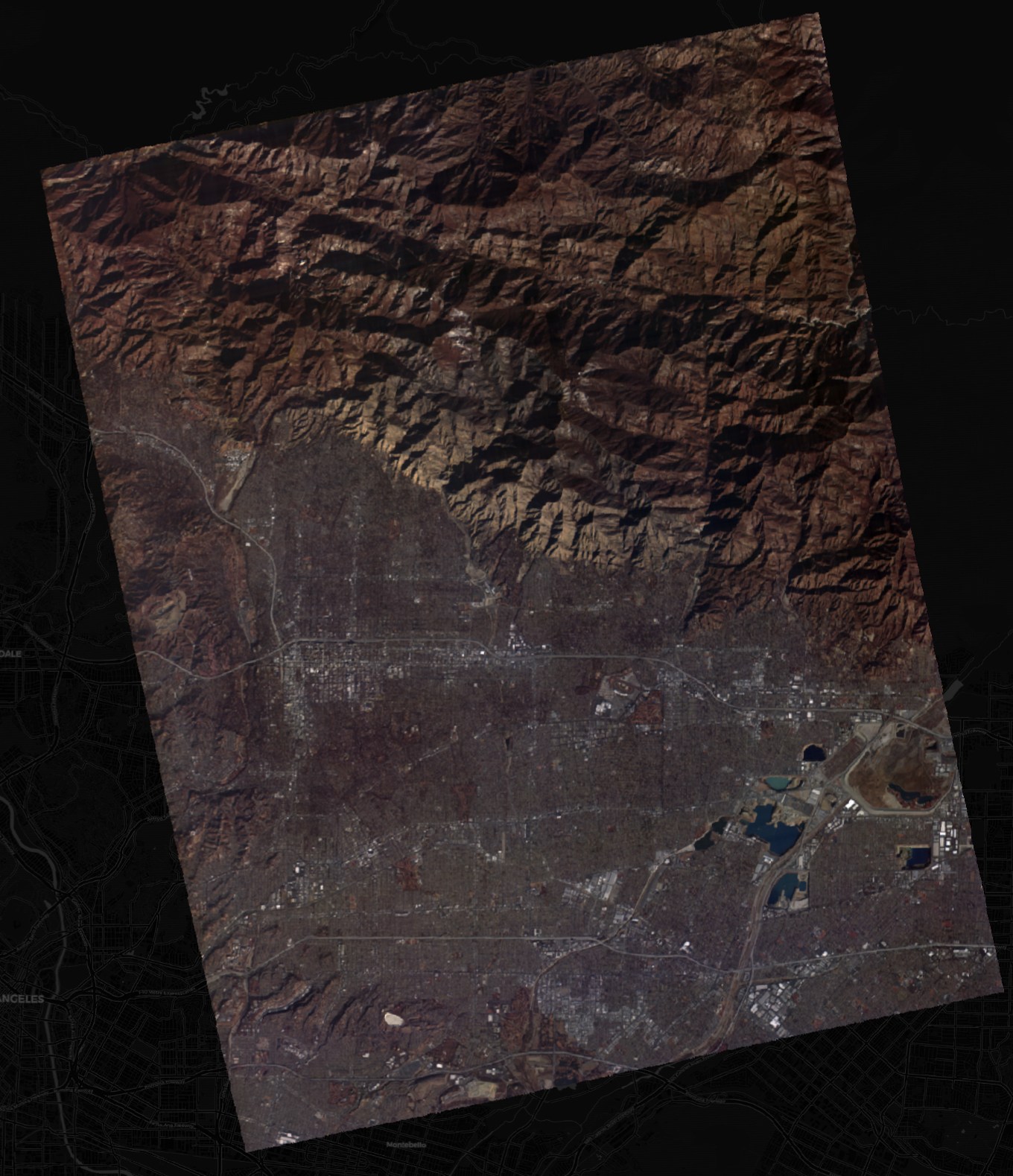
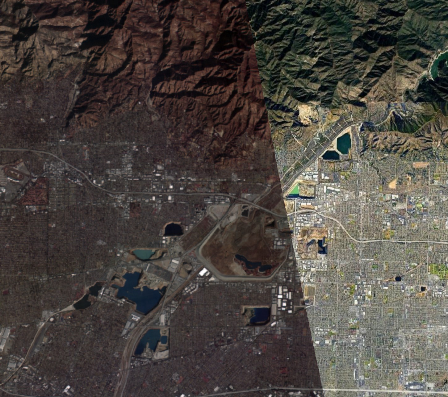
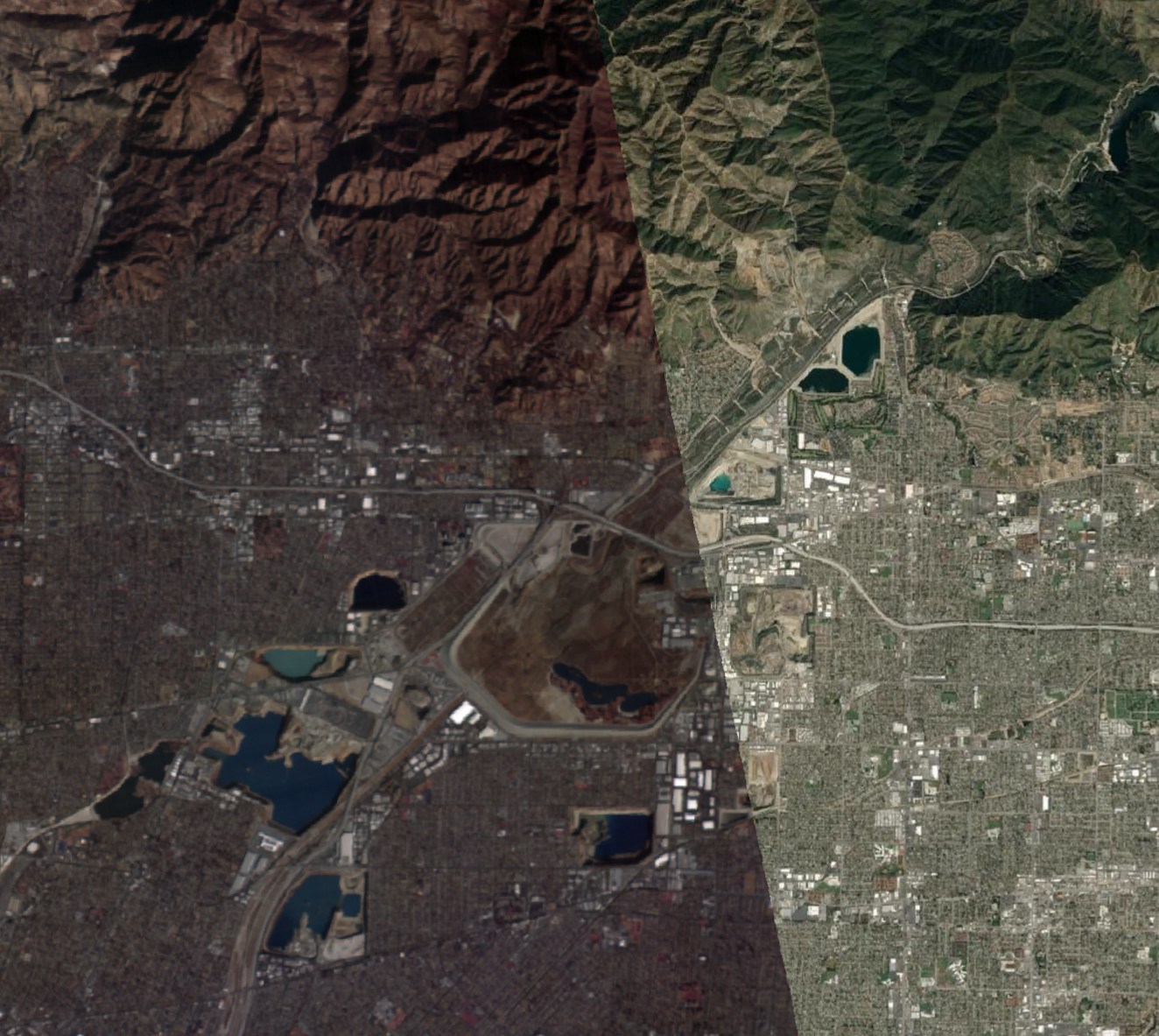
Below is a 23 x 30 KM image of Los Angeles.
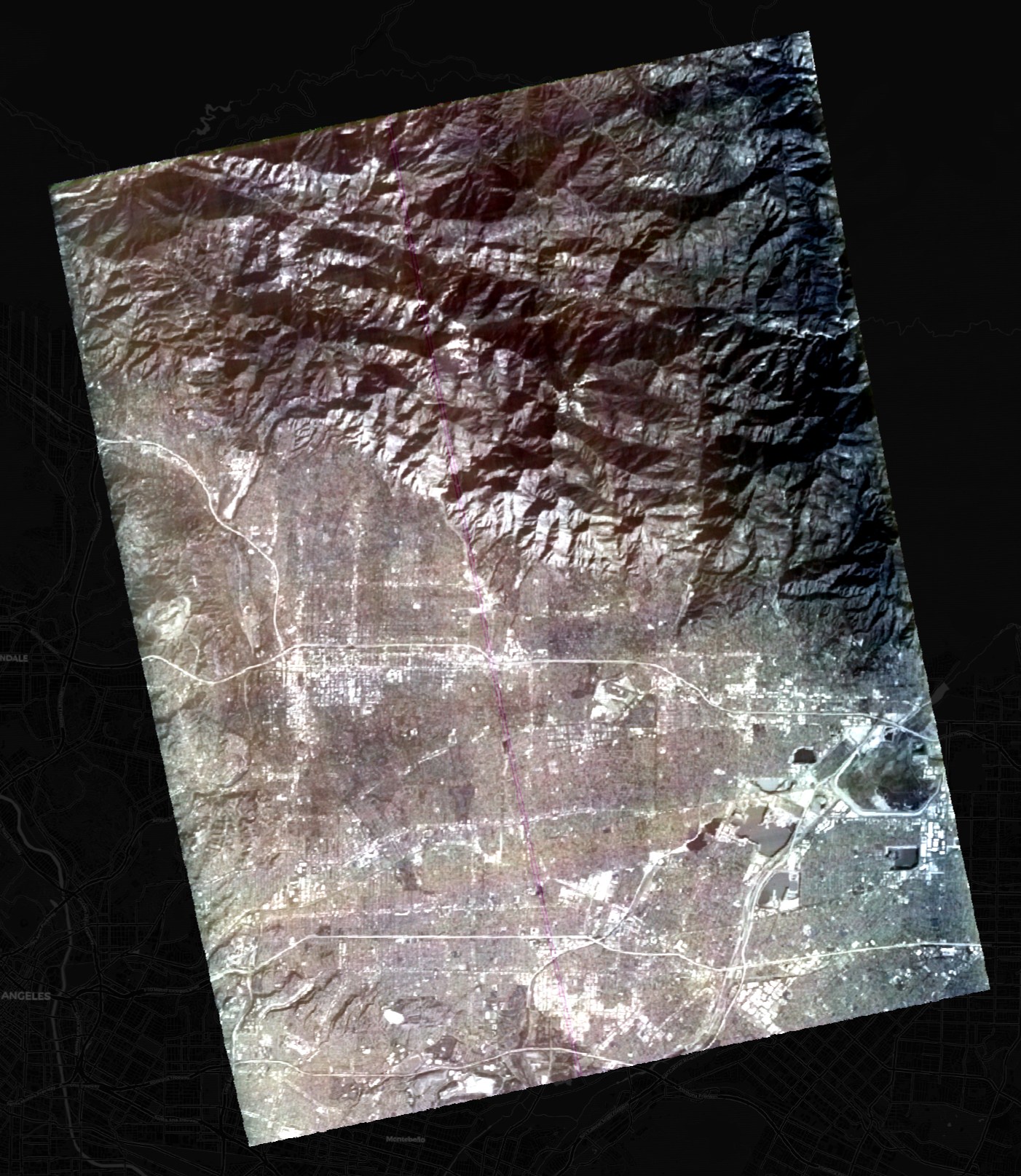
This is its metadata for reference.
$ echo "SELECT id,
               mapbox.json.address AS mapbox,
               properties::JSON AS properties
        FROM   imagery
        WHERE  assets::JSON LIKE '%001_20250124T171659_0bb0a026%'" \
    | ~/duckdb -json wyvern.duckdb \
    | jq -S .
[
  {
    "id": "wyvern_dragonette-001_20250124T171659_0bb0a026",
    "mapbox": "1330 Riviera Drive, Pasadena, California 91107, United States",
    "properties": {
      "constellation": "Dragonette",
      "created": "2025-01-26 03:03:59",
      "datetime": "2025-01-24T17:17:01.576537Z",
      "end_datetime": "2025-01-24T17:17:03.752084Z",
      "eo:cloud_cover": 45.79,
      "gsd": 5.26,
      "instruments": [
        "VNIR Hyperspectral Imaging Sensor"
      ],
      "license": "other",
      "platform": "Dragonette-001",
      "processing:facility": "Wyvern",
      "processing:level": "L1B",
      "processing:version": "1.3",
      "product_type": "hyperspectral",
      "proj:code": "EPSG:4326",
      "proj:shape": [
        6161,
        7459
      ],
      "providers": [
        {
          "name": "Wyvern Inc.",
          "roles": [
            "licensor",
            "producer",
            "processor"
          ],
          "url": "https://www.wyvern.space/"
        }
      ],
      "sat:platform_international_designator": "2023-054AZ",
      "sensor_mode": "strip",
      "sensor_type": "optical",
      "start_datetime": "2025-01-24T17:16:59.400989Z",
      "updated": "2025-01-26 03:03:59",
      "view:azimuth": 71.35445795857429,
      "view:incidence_angle": 16.779941471046186,
      "view:off_nadir": 18.07630168998292,
      "view:sun_azimuth": 136.73398188349992,
      "view:sun_elevation": 23.83740809718757,
      "wyvern:radiometric_resolution": "12"
    }
  }
]
The following bands are present in the above image.
Band_503nm  green   float32 0,0201 μm
Band_510nm  green   float32 0,0204 μm
Band_519nm  green   float32 0,0208 μm
Band_535nm  green   float32 0,0214 μm
Band_549nm  green   float32 0,022 μm
Band_570nm  green   float32 0,0228 μm
Band_584nm  yellow  float32 0,0234 μm
Band_600nm  yellow  float32 0,024 μm
Band_614nm  yellow  float32 0,0246 μm
Band_635nm  red     float32 0,0254 μm
Band_649nm  red     float32 0,026 μm
Band_660nm  red     float32 0,0264 μm
Band_669nm  red     float32 0,0268 μm
Band_679nm  red     float32 0,0272 μm
Band_690nm  red     float32 0,0276 μm
Band_699nm  red     float32 0,028 μm
Band_711nm  rededge float32 0,0284 μm
Band_722nm  rededge float32 0,0289 μm
Band_734nm  rededge float32 0,0294 μm
Band_750nm  rededge float32 0,03 μm
Band_764nm  rededge float32 0,0306 μm
Band_782nm  rededge float32 0,0313 μm
Band_799nm  nir     float32 0,032 μm
Most images contain 23 bands of data though there are four images in this feed that contain 31 bands.
$ for FILENAME in *.tiff; do
      echo `gdalinfo -json $FILENAME | jq -S '.stac."eo:bands"|length'`, $FILENAME
  done
23, wyvern_dragonette-001_20240608T144036_fa4c4f71.tiff
23, wyvern_dragonette-001_20240614T043114_805f0bb7.tiff
23, wyvern_dragonette-001_20240620T145630_2d5d0eef.tiff
23, wyvern_dragonette-001_20240628T062939_5fce57a3.tiff
23, wyvern_dragonette-001_20240703T171837_4c406dd3.tiff
23, wyvern_dragonette-001_20240709T145146_1e79473a.tiff
23, wyvern_dragonette-001_20240728T084002_5e95f389.tiff
23, wyvern_dragonette-001_20240802T063254_fe587307.tiff
23, wyvern_dragonette-001_20240806T172508_6b59089b.tiff
23, wyvern_dragonette-001_20240808T073501_51b92993.tiff
23, wyvern_dragonette-001_20240808T171453_20e65134.tiff
23, wyvern_dragonette-001_20240811T083914_08c61457.tiff
23, wyvern_dragonette-001_20240816T065054_0e692903.tiff
23, wyvern_dragonette-001_20240823T172127_4ef5c7ec.tiff
23, wyvern_dragonette-001_20240902T015820_c8ba843e.tiff
23, wyvern_dragonette-001_20240924T043743_be250f77.tiff
23, wyvern_dragonette-001_20240924T060726_6131fb18.tiff
23, wyvern_dragonette-001_20240930T070744_08fd7f5a.tiff
23, wyvern_dragonette-001_20241003T001114_b9b1a0b8.tiff
23, wyvern_dragonette-001_20241024T092200_c874e0e3.tiff
23, wyvern_dragonette-001_20241026T073007_1f933ec9.tiff
23, wyvern_dragonette-001_20241104T173856_870d7461.tiff
23, wyvern_dragonette-001_20241107T060700_4e89ebe5.tiff
23, wyvern_dragonette-001_20241219T073000_833394ce.tiff
23, wyvern_dragonette-001_20250101T072826_f3aa9cc0.tiff
23, wyvern_dragonette-001_20250123T172439_ec97451b.tiff
23, wyvern_dragonette-001_20250124T171659_0bb0a026.tiff
23, wyvern_dragonette-001_20250127T021633_c94c1fd6.tiff
23, wyvern_dragonette-001_20250202T013329_a6b233a1.tiff
31, wyvern_dragonette-003_20241224T002812_069c301b.tiff
31, wyvern_dragonette-003_20241229T103412_4fb7ca06.tiff
31, wyvern_dragonette-003_20241229T165203_12324bcb.tiff
31, wyvern_dragonette-003_20250128T005455_e8a5c3ba.tiff
Remapping Bands
If you open the properties for the above image's layer in QGIS and select the "Symbology" tab, you can re-map the bands being used for the red, green and blue channels being rendered. Try the following:
- Red band: "Band 15: Band_690"
- Green band: "Band 08: Band_600"
- Blue band: "Band 03: Band_519"
Under the "Min / Max Value Settings" section, check the radio button next to "Min / max".
Below is what the settings should look like:
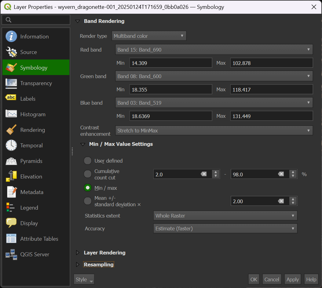
Hit "Apply" and the image should look more natural.
Below is a comparison to Bing's imagery for this area.
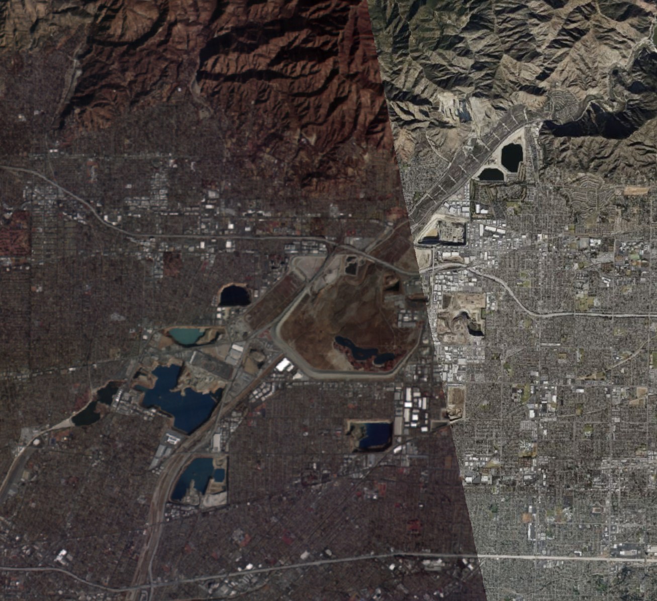
Below is a comparison to Esri's imagery for this area.
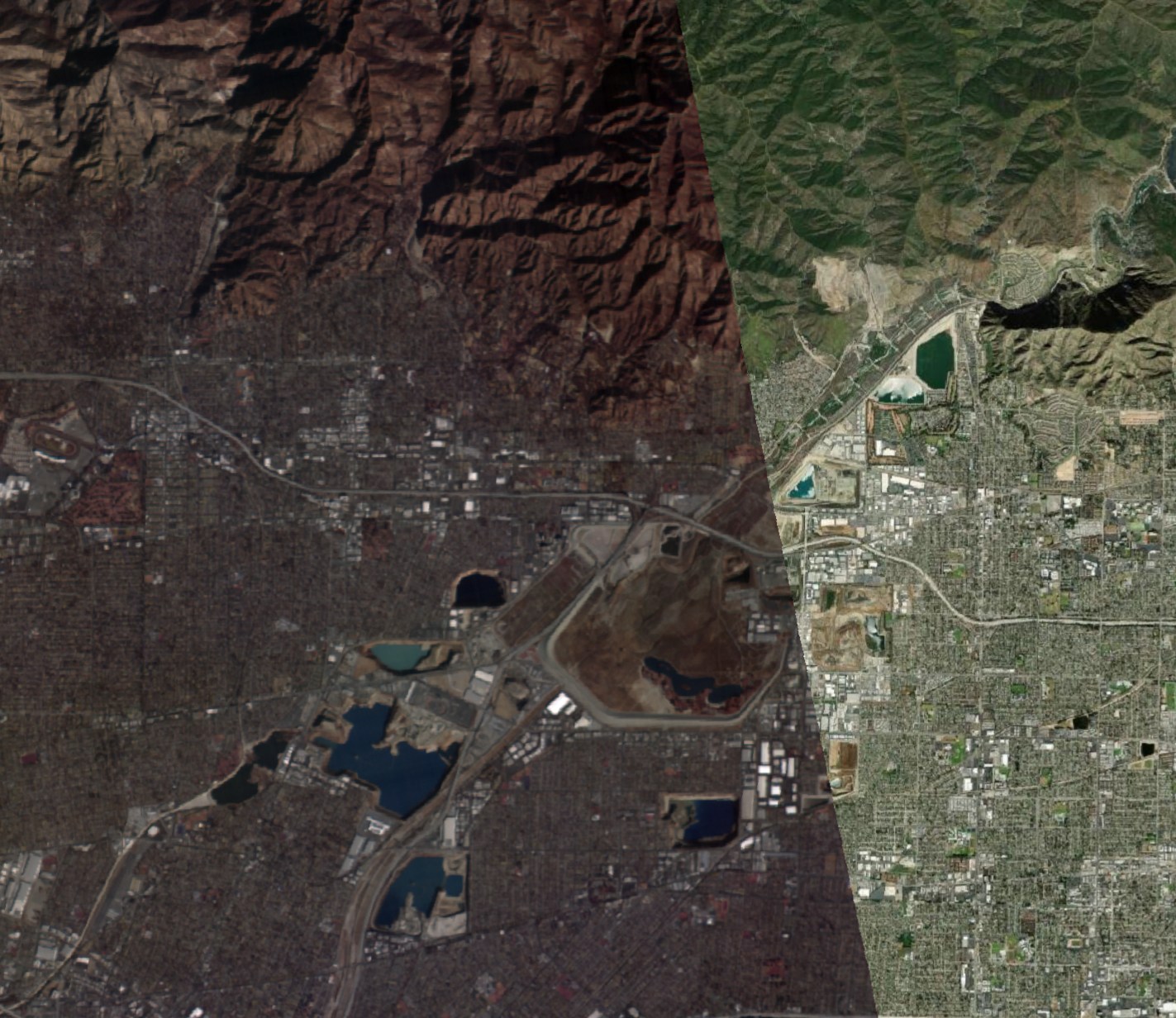
Below is a comparison to Google's imagery for this area.
Below is a comparison to Yandex's imagery for this area.
STAC Support in QGIS
QGIS 3.42 was released a few weeks ago and now has STAC catalog integration.
From the Layer Menu, click Add Layer -> Add Layer from STAC Catalog.
Give the layer the name "wyvern" and paste in the following URL:
https://wyvern-prod-public-open-data-program.s3.ca-central-1.amazonaws.com/catalog.json
Below is what the fields should look like.
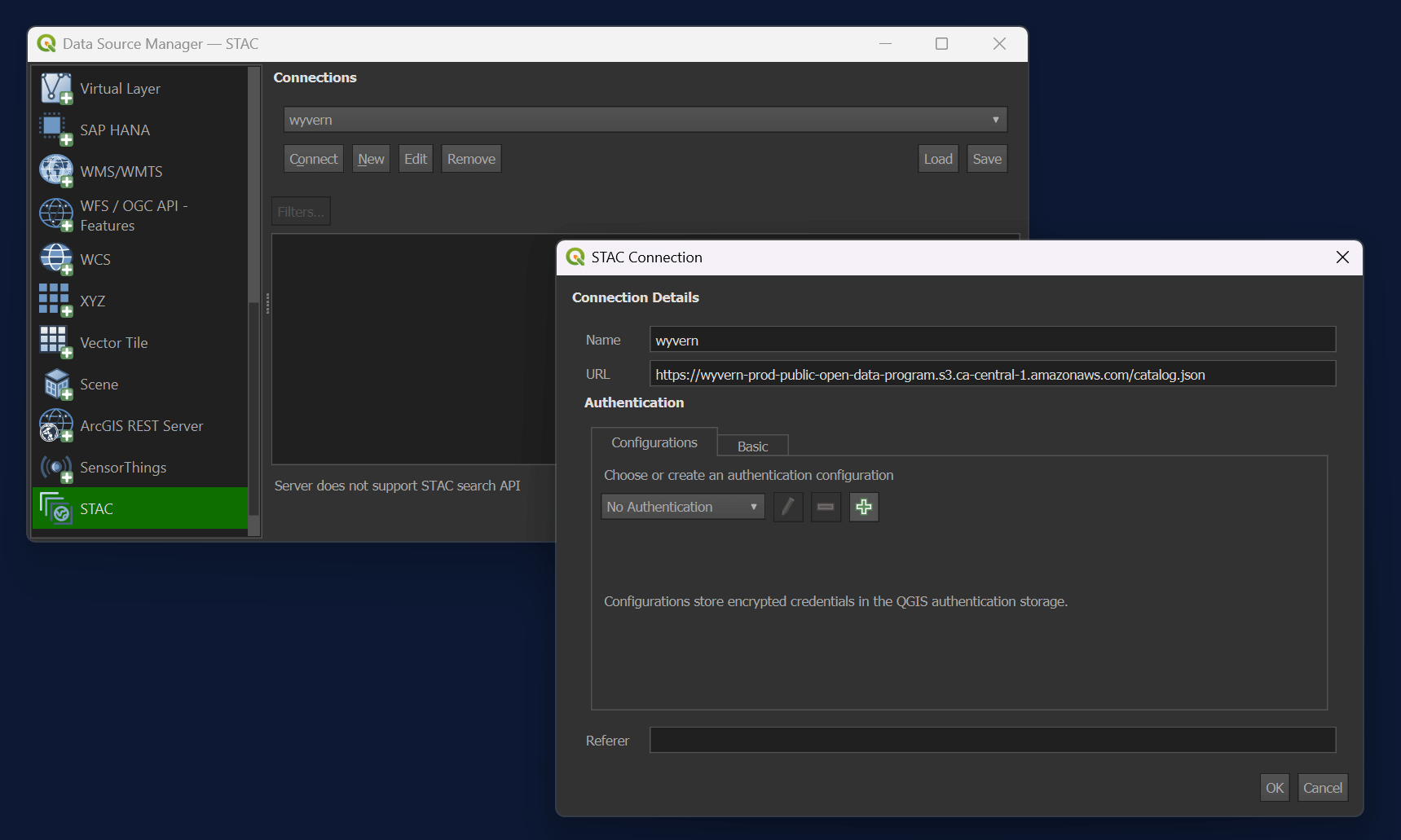
Click OK, then Close on the next dialog and return to the main UI. Don't click the connect button as you'll receive an error message and it isn't needed for this feed.
Click the View Menu -> Panels -> Browser Panel. You should see a STAC item appear in that panel and underneath you should be able to browse the various collections Wyvern offer.
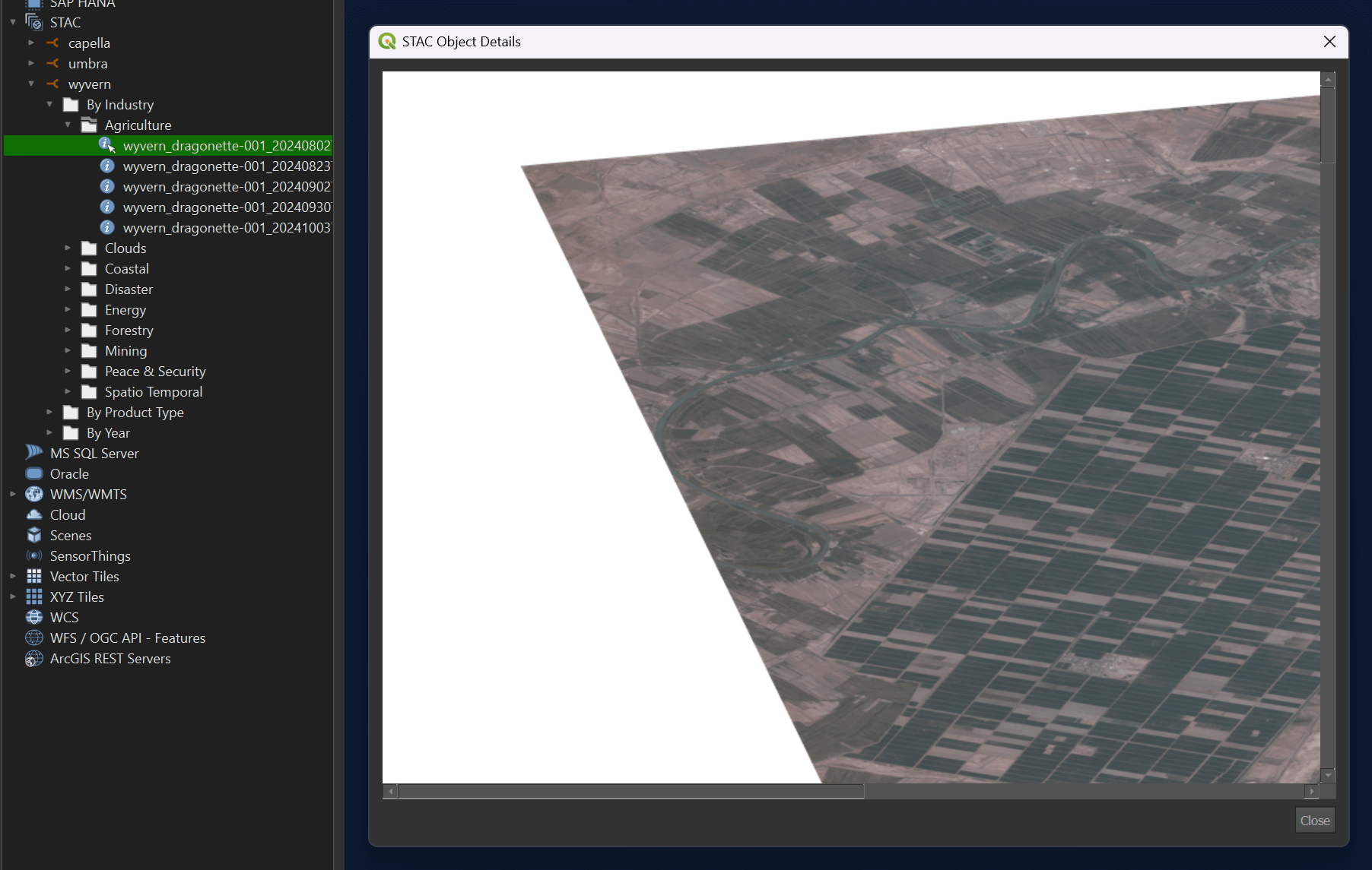
Right clicking any asset lets you both see a preview and details on the imagery. You can also download the imagery to your machine and into your QGIS project.