Since November, Overture Maps has been publishing global, open geospatial datasets every month. They've also expanded the topics they cover from building footprints and road networks to address lists and AI-generated land use data.
They've managed to get several major geospatial software, data providers and the OpenStreetMap (OSM) community to come together to produce these datasets and provide them publicly free of charge.
The first release of their datasets a year ago was a Protocols Buffer file. This format makes it difficult to search for and extract data of interest. Its 90 GB+ file size also made it challenging for desktop software to work with.
Since then, they've moved to shipping data in Parquet format. In April, they began spatially sorting the data so that the files could be compressed better and extracting data for specific towns and cities became much quicker.
This month, they announced an Explorer web application which will let you inspect their datasets in a web browser. This web app is serverless and uses JavaScript to fetch map data from 371 GB worth of PM Tiles on AWS Cloudfront. When you view a location, the web app is smart enough to only download the data needed to render what you're looking at. Overture has stated they'll be shipping these PM Tiles files in future releases of their datasets.
In this post, I'll walk through some of the newer datasets Overture has released this year as well as go over the evolution of their building footprints.
My Workstation
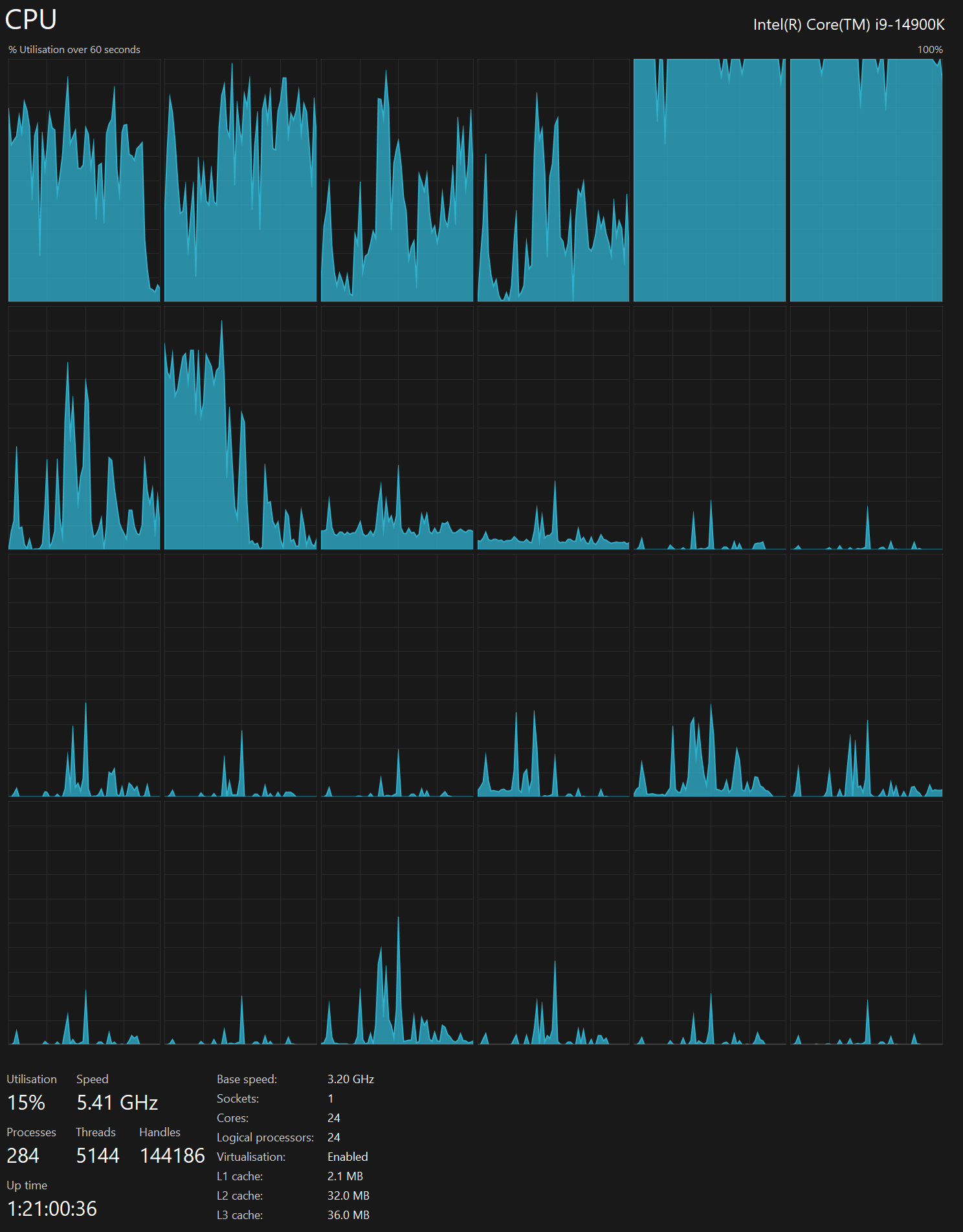
I'm using a 6 GHz Intel Core i9-14900K CPU. It has 8 performance cores and 16 efficiency cores with a total of 32 threads and 32 MB of L2 cache. It has a liquid cooler attached and is housed in a spacious, full-sized, Cooler Master HAF 700 computer case. I've come across videos on YouTube where people have managed to overclock the i9-14900KF to 9.1 GHz.
The system has 96 GB of DDR5 RAM clocked at 6,000 MT/s and a 5th-generation, Crucial T700 4 TB NVMe M.2 SSD which can read at speeds up to 12,400 MB/s. There is a heatsink on the SSD to help keep its temperature down. This is my system's C drive.
The system is powered by a 1,200-watt, fully modular, Corsair Power Supply and is sat on an ASRock Z790 Pro RS Motherboard.
I'm running Ubuntu 22 LTS via Microsoft's Ubuntu for Windows on Windows 11 Pro. In case you're wondering why I don't run a Linux-based desktop as my primary work environment, I'm still using an Nvidia GTX 1080 GPU which has better driver support on Windows and I use ArcGIS Pro from time to time which only supports Windows natively.
Installing Prerequisites
I'll be using Python and a few other tools to help analyse the data in this post.
$ sudo apt update
$ sudo apt install \
    aws-cli \
    jq \
    python3-pip \
    python3-virtualenv \
    unzip
I'll set up a Python Virtual Environment and install osm_split's dependencies. This tool makes it much easier to break apart OSM data into named files with individual fields of metadata.
$ virtualenv ~/.osm
$ source ~/.osm/bin/activate

$ git clone https://github.com/marklit/osm_split
$ python -m pip install -r osm_split/requirements.txt
I'll also use DuckDB, along with its H3, JSON, Parquet and Spatial extensions, in this post.
$ cd ~
$ wget -c https://github.com/duckdb/duckdb/releases/download/v1.0.0/duckdb_cli-linux-amd64.zip
$ unzip -j duckdb_cli-linux-amd64.zip
$ chmod +x duckdb
$ ~/duckdb
INSTALL h3 FROM community;
INSTALL json;
INSTALL parquet;
INSTALL spatial;
I'll set up DuckDB to load every installed extension each time it launches.
$ vi ~/.duckdbrc
.timer on
.width 180
LOAD h3;
LOAD json;
LOAD parquet;
LOAD spatial;
The maps in this post were rendered with QGIS version 3.38.0. QGIS is a desktop application that runs on Windows, macOS and Linux. The application has grown in popularity in recent years and has ~15M application launches from users around the world each month.
I used QGIS' Tile+ plugin to add geospatial context with Esri's World Imagery and CARTO's Basemaps to the maps.
Downloading Natural Earth Data
I'll use Natural Earth's Global Geospatial dataset to help me identify populated places around the world. The following downloaded version 5.1.2 they released in May 2022.
$ mkdir -p ~/naturalearth

$ for DATASET in cultural physical raster; do
      cd ~/naturalearth
      aws s3 sync \
            --no-sign-request \
            s3://naturalearth/10m_$DATASET/ \
            10m_$DATASET/

      cd 10m_$DATASET/
      ls *.zip | xargs -n1 -P4 -I% unzip -qn %
  done
Downloading Overture's Data
Overture tends to publish a new dataset in the middle of each month. The following will list each publication they've made.
$ aws s3 --no-sign-request ls s3://overturemaps-us-west-2/release/
PRE 2023-04-02-alpha/
PRE 2023-07-26-alpha.0/
PRE 2023-10-19-alpha.0/
PRE 2023-11-14-alpha.0/
PRE 2023-12-14-alpha.0/
PRE 2024-01-17-alpha.0/
PRE 2024-02-15-alpha.0/
PRE 2024-03-12-alpha.0/
PRE 2024-04-16-beta.0/
PRE 2024-05-16-beta.0/
PRE 2024-06-13-beta.0/
PRE 2024-06-13-beta.1/
PRE 2024-07-22.0/
I'll download the 517 GB of parquet data in this month's publication.
$ aws s3 --no-sign-request sync \
    s3://overturemaps-us-west-2/release/2024-07-22.0 \
    ~/2024_07
It is possible to work with Overture's Parquet files on S3 rather than storing them locally but I found querying their data on an SATA-backed SSD was ~5x faster than off of S3 on my 500 Mbps broadband connection.
Breaking Down Overture
I'll download a JSON-formatted listing of every object in Overture's S3 bucket.
$ aws --no-sign-request \
      --output json \
      s3api \
      list-objects \
      --bucket overturemaps-us-west-2 \
      --max-items=1000000 \
    | jq -c '.Contents[]' \
    > overturemaps.s3.json
As of this writing, there are 11.4K files and ~4.5 TB of data across all their releases.
$ echo "Total objects: " `wc -l overturemaps.s3.json | cut -d' ' -f1`, \
       " TB: " `jq .Size overturemaps.s3.json | awk '{s+=$1}END{print s/1024/1024/1024/1024}'`
Total objects: 11474, TB: 4.49255
The following breaks down how many GB make up each theme within each of their releases.
$ ~/duckdb
CREATE OR REPLACE TABLE s3 AS
    SELECT *,
           SPLIT(Key, '/')[1]                        AS section,
           SPLIT(Key, '/')[2]                        AS release,
           REPLACE(SPLIT(Key, '/')[3], 'theme=', '') AS theme,
           REPLACE(SPLIT(Key, '/')[4], 'type=', '')  AS theme_type
    FROM   READ_JSON('overturemaps.s3.json')
    WHERE  Key NOT LIKE '%planet%'
    AND    Key NOT LIKE '%_SUCCESS%'
    AND    Key NOT LIKE '%building-extracts%'
    AND    section = 'release';

WITH a AS (
    SELECT   theme,
             release,
             ROUND(SUM(Size) / 1024 / 1024 / 1024)::INT sum_size
    FROM     s3
    GROUP BY 1, 2
)
PIVOT    a
ON       theme
USING    SUM(sum_size)
ORDER BY release;
┌────────────────────┬───────────┬────────┬────────┬───────────┬───────────┬────────┬────────────────┐
│      release       │ addresses │ admins │  base  │ buildings │ divisions │ places │ transportation │
│      varchar       │  int128   │ int128 │ int128 │  int128   │  int128   │ int128 │     int128     │
├────────────────────┼───────────┼────────┼────────┼───────────┼───────────┼────────┼────────────────┤
│ 2023-07-26-alpha.0 │           │      1 │        │       110 │           │      8 │             82 │
│ 2023-10-19-alpha.0 │           │      2 │     61 │       176 │           │      7 │             81 │
│ 2023-11-14-alpha.0 │           │      2 │     59 │       154 │           │      6 │             76 │
│ 2023-12-14-alpha.0 │           │      2 │     52 │       231 │           │      5 │             63 │
│ 2024-01-17-alpha.0 │           │      2 │     53 │       232 │           │      6 │             63 │
│ 2024-02-15-alpha.0 │           │      3 │     50 │       232 │           │      5 │             65 │
│ 2024-03-12-alpha.0 │           │      3 │     50 │       232 │           │      5 │             65 │
│ 2024-04-16-beta.0  │           │      3 │     51 │       196 │         4 │      4 │             56 │
│ 2024-05-16-beta.0  │           │      3 │    147 │       197 │         4 │      4 │             58 │
│ 2024-06-13-beta.0  │           │      3 │    141 │       212 │         4 │      5 │             58 │
│ 2024-06-13-beta.1  │           │      3 │    141 │       212 │         3 │      5 │             58 │
│ 2024-07-22.0       │         6 │        │    142 │       213 │         4 │      5 │             58 │
├────────────────────┴───────────┴────────┴────────┴───────────┴───────────┴────────┴────────────────┤
│ 12 rows                                                                                  8 columns │
└────────────────────────────────────────────────────────────────────────────────────────────────────┘
The buildings dataset hovered around 232 GB between December and March. In April it dropped to 196 GB. This would have been due to their migration to spatially sorting their Parquet files. This made it much easier for ZStandard to compress the data. Since then, the dataset has been steadily growing.
Within each theme, there are one or more "types". Below are the sizes of each type for this month's release.
Size (GB) | theme          | type
----------|----------------|------------------
    363   | buildings      | building
     84   | base           | land_cover
     46   | transportation | segment
     21   | base           | land
     19   | base           | water
     13   | transportation | connector
     13   | base           | land_use
      6.5 | addresses      | address
      6.3 | base           | infrastructure
      4.6 | places         | place
      2.8 | divisions      | division_area
      0.3 | divisions      | division
      0.3 | divisions      | division_boundary
      0.3 | buildings      | building_part
Buildings are the majority of the release at 363 GB compressed.
Transport makes up 59 GB with segments making up 46 GB of that theme's footprint.
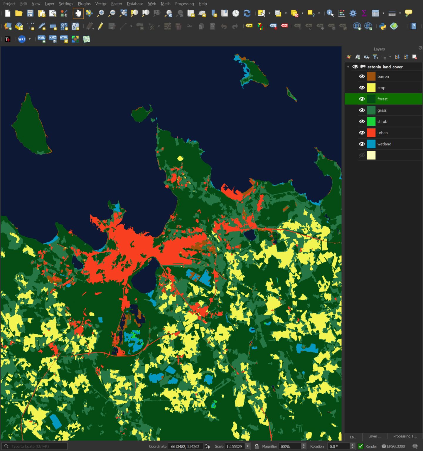
The base theme is 143 GB with land cover taking up over half of that theme's footprint. Below is a screenshot of the land use data for Tallinn, Estonia.
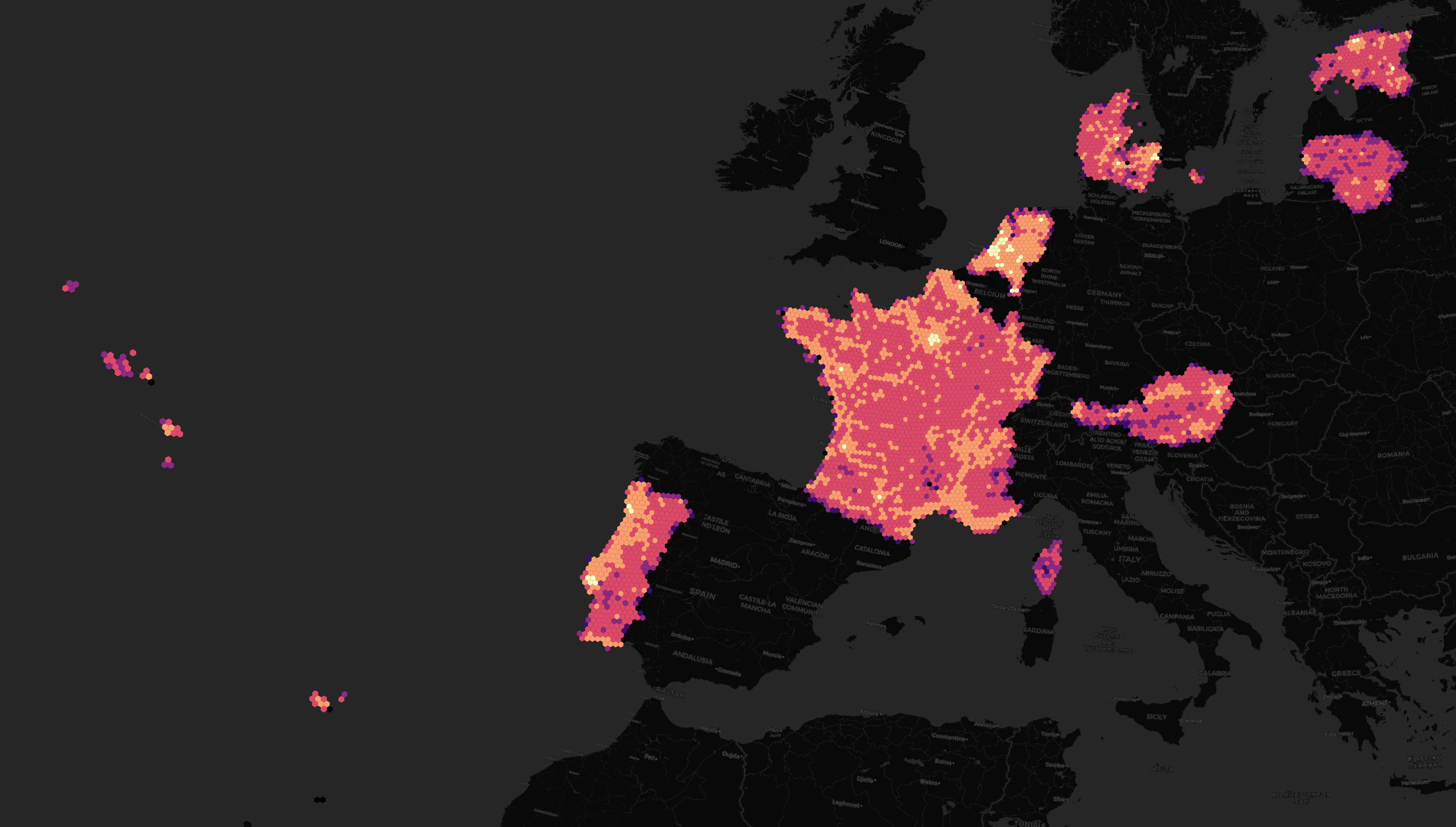
Addresses
This month's release now includes addresses for 14 countries, including the US. Below is a heatmap of how many addresses they have in each state. This dataset is still a work in progress and there are a bunch of gaps in the dataset.
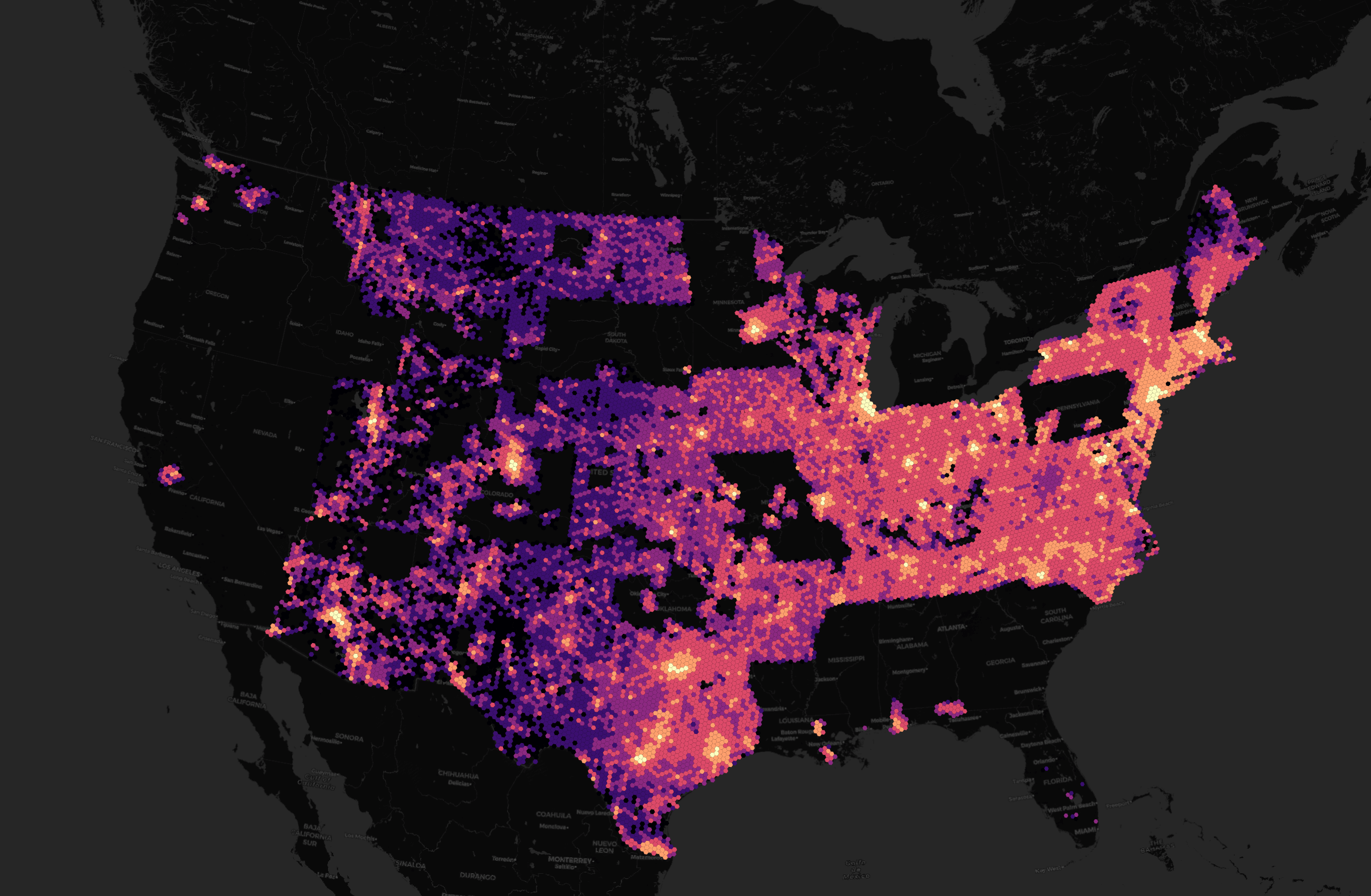
I've seen clients spending huge sums of money on US address data and it is expensive. Their efforts towards producing a free dataset will remove a lot of financial and technical overhead in future geospatial projects.
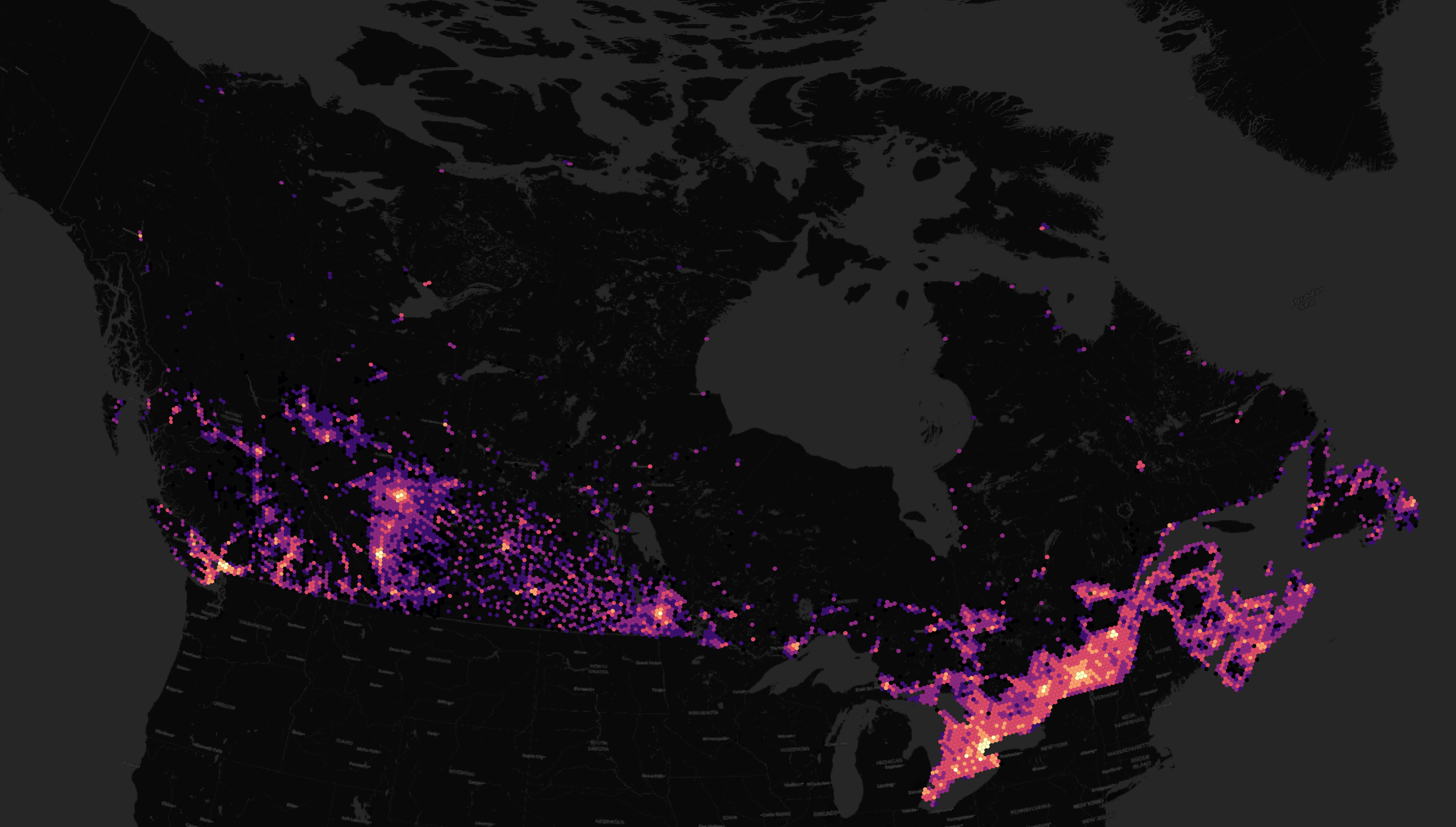
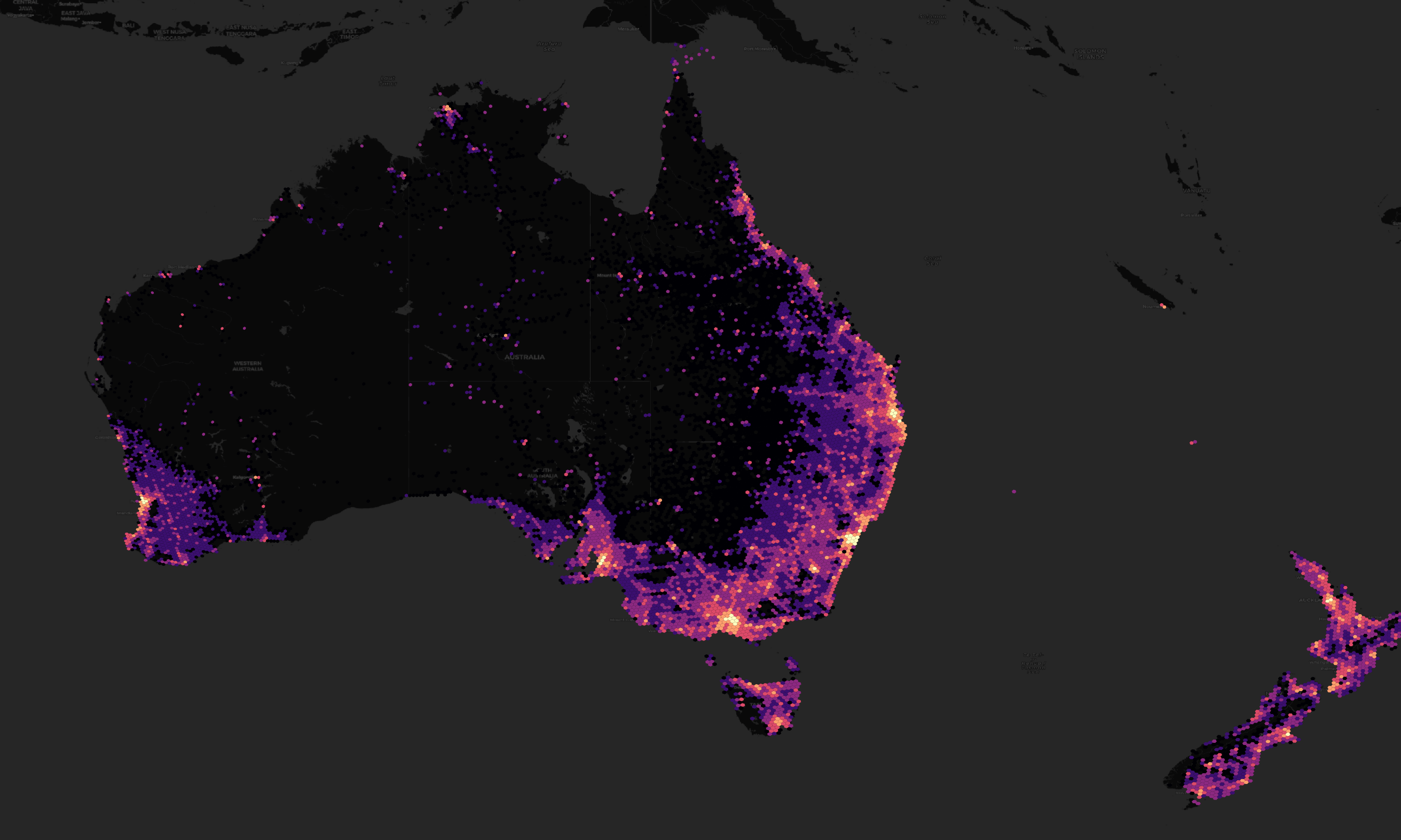
The address density for Canada, Australia and New Zealand match their population densities pretty well.
A handful of EU member states, including Estonia, are represented in this addresses dataset as well.
The addresses have been sourced from the OpenAddresses project and often originated from national land boards.
$ cd ~/2024_07/theme\=addresses/type\=address/
$ ~/duckdb
SELECT   country,
         COUNT(*) AS num_addrs,
         sources->0->'dataset' AS source
FROM     READ_PARQUET('*')
WHERE    country != 'US'
GROUP BY 1, 3
ORDER BY 1, 2 DESC;
┌─────────┬───────────┬──────────────────────────────────────────────────────────┐
│ country │ num_addrs │                          source                          │
│ varchar │   int64   │                           json                           │
├─────────┼───────────┼──────────────────────────────────────────────────────────┤
│ AT      │   2492155 │ "OpenAddresses/Bundesamt für Eich- und Vermessungswesen" │
│ AU      │  15608317 │ "OpenAddresses/Geosacape Australia"                      │
│ CA      │  16457790 │ "OpenAddresses/Statistics Canada"                        │
│ CO      │   7786046 │ "OpenAddresses/AddressForAll/DANE"                       │
│ DK      │   3918869 │ "OpenAddresses/DAWA"                                     │
│ EE      │   2211770 │ "OpenAddresses/MAA-AMET"                                 │
│ FR      │  26041499 │ "OpenAddresses/adresse.data.gouv.fr"                     │
│ LT      │   1036251 │ "OpenAddresses/Registrų Centras"                         │
│ LU      │    164415 │ "OpenAddresses/data.public.lu"                           │
│ MX      │  30278896 │ "OpenAddresses/AddressForAll/INEGI"                      │
│ NL      │   9750341 │ "OpenAddresses/NGR"                                      │
│ NZ      │   2348842 │ "OpenAddresses/LINZ"                                     │
│ PT      │   5911139 │ "OpenAddresses/INE"                                      │
├─────────┴───────────┴──────────────────────────────────────────────────────────┤
│ 13 rows                                                              3 columns │
└────────────────────────────────────────────────────────────────────────────────┘
I've had to exclude the US from the above query as DuckDB isn't happy with some of the JSON in the source column of the US dataset.
Invalid Input Error: Malformed JSON at byte 85 of input: unexpected character. Input: [{"property":"","dataset":"NAD","record_id":nul...
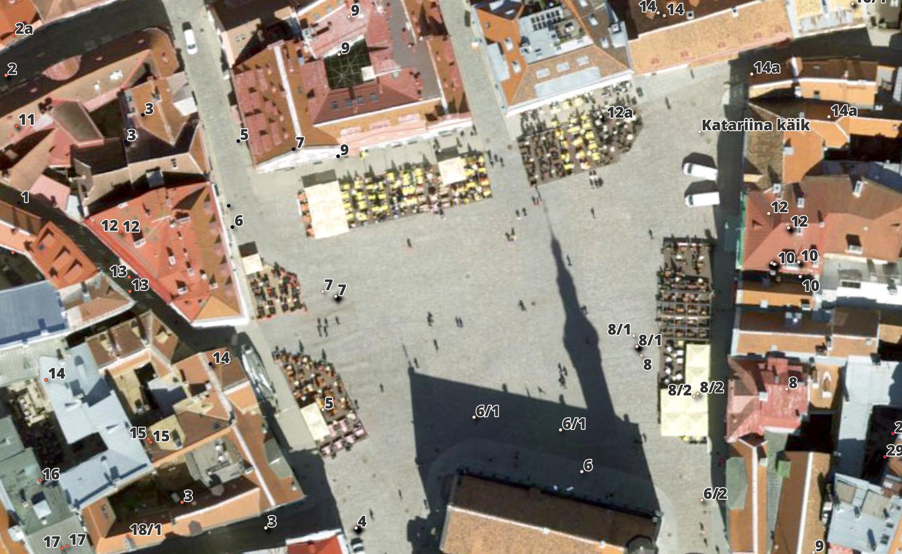
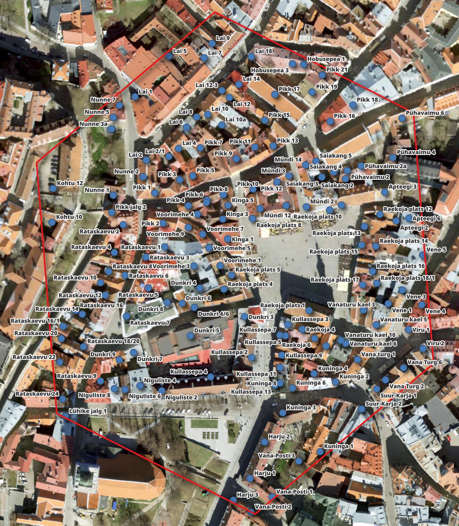
I haven't closely examined every country's addresses yet but the Estonian ones have a lot of duplicates and misplaced locations. The following screenshot is from Raekoja plats in Tallinn's Old Town.
Below, I'll investigate some alternative ways to produce an Estonian address list.
Estonia's Open Geospatial Portal
Estonia's Land Board has an Open Geospatial Portal. I downloaded the addresses for the whole of Estonia. They are shipped as a 124 MB ZIP containing a 2.2M-line, 925 MB CSV file. I've used iconv to fix up some of the Unicode in the CSV.
$ cd ~
$ wget https://xgis.maaamet.ee/adsavalik/valjav6te/1_26072024_03805.zip
$ unzip 1_26072024_03805.zip
$ iconv -f latin1 \
        -t utf-8 \
        1_26072024_03805_1.csv \
    > 1_26072024_03805_1.utf8.csv
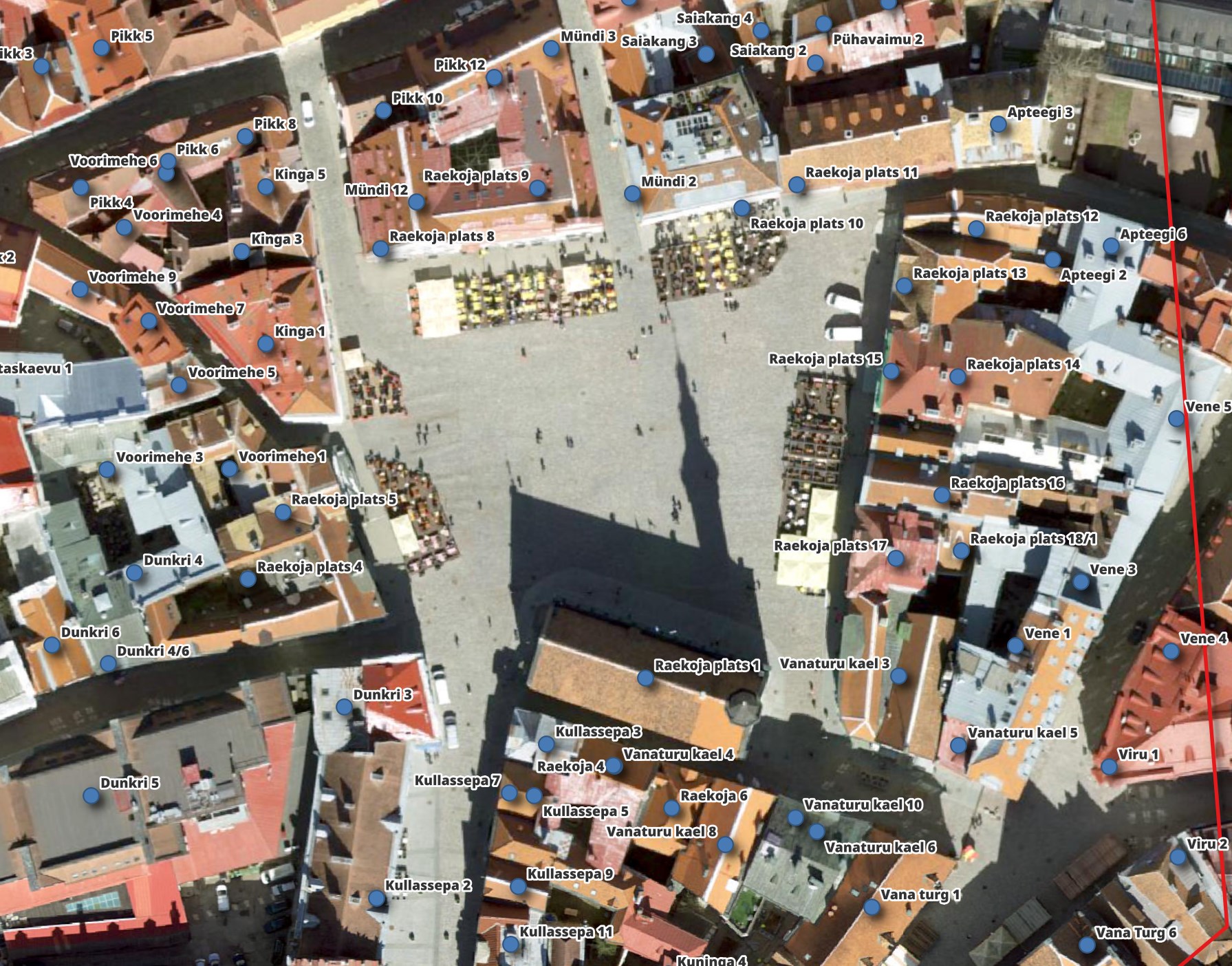
Below is a screenshot of the Estonian Land Board's data for Raekoja plats.
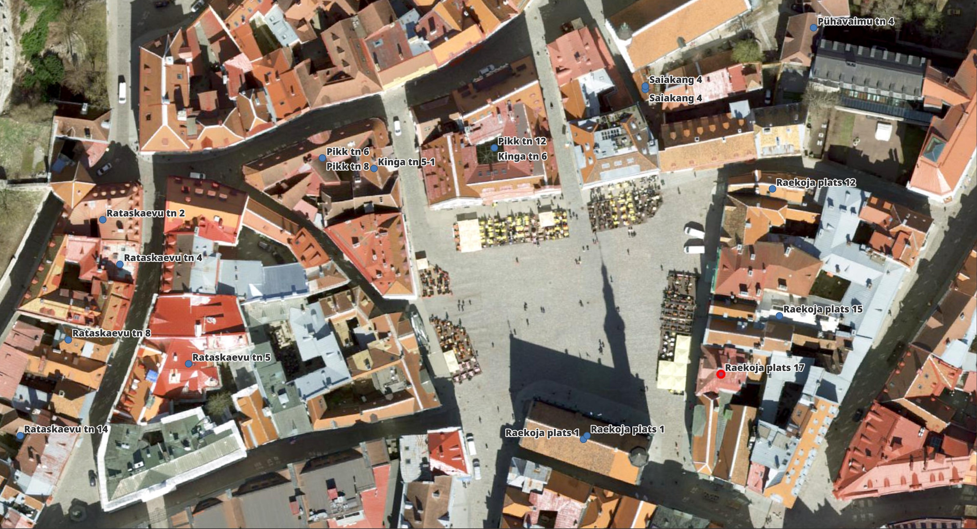
None of their labels are misplaced but many addresses are missing. There are also some points which are for the same address but have differing metadata. I used QGIS to export the above CSV to a GeoPackage (GPKG) file. I'll examine the resulting GPKG file with DuckDB.
Below are the fields that differ for the address 'Raekoja plats 1'.
$ ~/duckdb
SELECT ADOB_ID,
       ADS_OID,
       ADOB_LIIK,
       ORIG_TUNNUS,
       ADS_KEHTIV,
       VIITEPUNKT_X,
       VIITEPUNKT_Y,
       geom
FROM   ST_READ('1_26072024_03805_1.gpkg')
WHERE  LAHIAADRESS = 'Raekoja plats 1';
┌─────────┬────────────┬───────────┬────────────────┬─────────────────────┬──────────────┬──────────────┬────────────────────────┐
│ ADOB_ID │  ADS_OID   │ ADOB_LIIK │  ORIG_TUNNUS   │     ADS_KEHTIV      │ VIITEPUNKT_X │ VIITEPUNKT_Y │          geom          │
│  int32  │  varchar   │  varchar  │    varchar     │       varchar       │    int32     │    int32     │        geometry        │
├─────────┼────────────┼───────────┼────────────────┼─────────────────────┼──────────────┼──────────────┼────────────────────────┤
│ 6634269 │ CU00444091 │ CU        │ 78401:101:0540 │ 18.10.2014 07:47:04 │       542293 │      6589032 │ POINT (542293 6589032) │
│ 6419941 │ ME00653209 │ ME        │ 101036399      │ 17.10.2014 19:15:18 │       542294 │      6589033 │ POINT (542294 6589033) │
└─────────┴────────────┴───────────┴────────────────┴─────────────────────┴──────────────┴──────────────┴────────────────────────┘
The Land Board has a decent explanation of their record policy. The short of it is that a single address can have more than one record. Using the above CSV for generating a distinct building address list of Estonia will produce an incomplete list of addresses and come with many edge cases that would have to be taken into account.
Addresses from OpenStreetMap
OSM does a good job of listing each address in Tallinn's Old Town.
I'll use GeoFabrik's latest release of the OSM data for Estonia and export the Old Town data into GPKG files. I'll be using an H3 hexagon filter to isolate the areas in and around Raekoja plats.
$ mkdir -p ~/geofabrik
$ cd ~/geofabrik

$ wget -c https://download.geofabrik.de/europe/estonia-latest.osm.pbf
$ python ~/osm_split/main.py \
        estonia-latest.osm.pbf \
        --only-h3=89089b1a283ffff
The osm_split tool I built will break up PBF files by geometry type and name of the type of structure. These are stored as GPKG files which have an R-Tree index which makes opening them up and exploring them in QGIS and other applications much quicker.
The files have names of what they represent which makes discovering data of interest much easier.
The key-value pairs in the original PBF files are broken up into individual fields in the GPKG file so they're as easy to work with as any database table. DuckDB can query them just like it could query any database.
The above produced 82 GPKG files.
$ find [a-z]*/ | grep gpkg$ | wc -l # 82
Below are a couple of the GPKG files produced.
$ find lines/ -type f | head
lines/barrier.gpkg
lines/building/apartments.gpkg
lines/building/church.gpkg
lines/building/commercial.gpkg
lines/building/government.gpkg
lines/building/historic.gpkg
lines/building/retail.gpkg
lines/building/service.gpkg
lines/building.gpkg
lines/grass.gpkg
I'll collect the centroid and address data in each of the GPKG files' records and save them to a JSONL file. Some files won't contain any address metadata so I've wrapped the extraction in an exception that ignores any errors around the assumption that all files should contain address metadata.
$ python3
import duckdb
from   pathlib import Path


sql = """SELECT DISTINCT ST_CENTROID(geom)::TEXT AS geom,
                         COLUMNS(c -> c LIKE 'addr%')
         FROM   ST_READ(?)"""

con = duckdb.connect(database=':memory:')
con.sql('INSTALL spatial; LOAD spatial;')

with open('recs.json', 'w') as f:
    for filename in Path('.').glob('**/*.gpkg'):
        # Ignore missing address data which will be reported like the
        # following:

        # Star expression "COLUMNS(list_filter(['barrier', 'colour',
        # 'material', 'geom'], (c -> (c ~~ 'addr%'))))" resulted in an
        # empty set of columns

        try:
            df = con.sql(sql, params=(str(filename),)).to_df()
        except duckdb.InvalidInputException:
            continue

        for rec in df.iloc():
            f.write(rec.to_json() + '\n')
I'll then produce a distinct list of addresses from the above using DuckDB. The following produced 153 addresses from the 532 records in the above JSON file.
$ ~/duckdb
COPY (
    WITH a AS (
        SELECT *,
               ROW_NUMBER() OVER (PARTITION BY LOWER("addr:street"),
                                               "addr:housenumber"
                                  ORDER BY geom) AS rn
        FROM   READ_JSON('recs.json')
        WHERE  LENGTH("addr:street")
        AND    LENGTH("addr:housenumber")
    )
    SELECT "addr:street"      AS street,
           "addr:housenumber" AS house_num,
           geom::geometry     AS geom
    FROM   a
    WHERE  rn = 1
) TO 'recs.gpkg'
  WITH (FORMAT GDAL,
        DRIVER 'GPKG',
        LAYER_CREATION_OPTIONS 'WRITE_BBOX=YES');
The above shows that pretty much every building within the hexagon has an address for each of its distinct properties. I've drawn the hexagon geospatial filter I used above on the map in red.
Below I'll zoom into Raekoja plats for a closer look.
Building Data
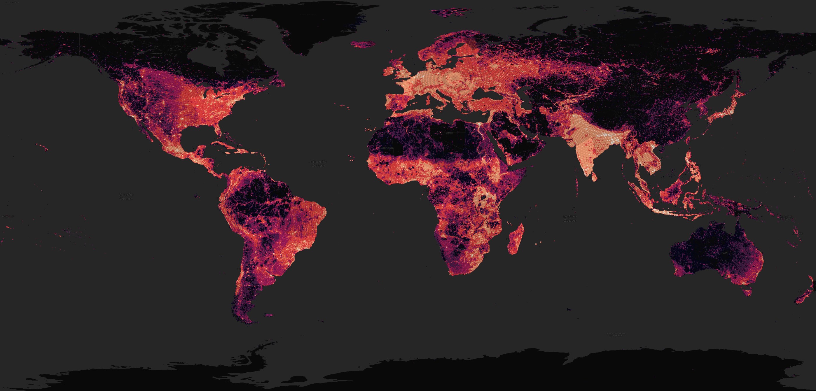
Overture uses many sources for their building data including OSM, Microsoft ML Buildings and Google Open Buildings. This has resulted in very good global coverage for their building footprint dataset. Below is a heatmap of building density in Overture's dataset.
I haven't found a way to get QGIS to render polygons that sit over the International Dateline nicely so I'll exclude any geometry anywhere near this area for the rendering below.
$ cd ~/2024_07/theme\=buildings/type\=building
$ ~/duckdb
COPY (
    WITH a AS (
        SELECT H3_CELL_TO_PARENT(
                    H3_STRING_TO_H3(SUBSTR(id, 0, 17)), 5) h3_val,
               COUNT(*) num_recs
        FROM   READ_PARQUET('*.parquet',
                            hive_partitioning=1)
        GROUP BY 1
    )
    SELECT H3_CELL_TO_BOUNDARY_WKT(h3_val)::GEOMETRY geom,
           num_recs
    FROM  a
    WHERE H3_CELL_TO_LNG(h3_val) > -175
    AND   H3_CELL_TO_LNG(h3_val) < 175
) TO 'buildings_h3.2024-07-22.gpkg'
    WITH (FORMAT GDAL,
          DRIVER 'GPKG',
          LAYER_CREATION_OPTIONS 'WRITE_BBOX=YES');
Spatially Sorted Datasets
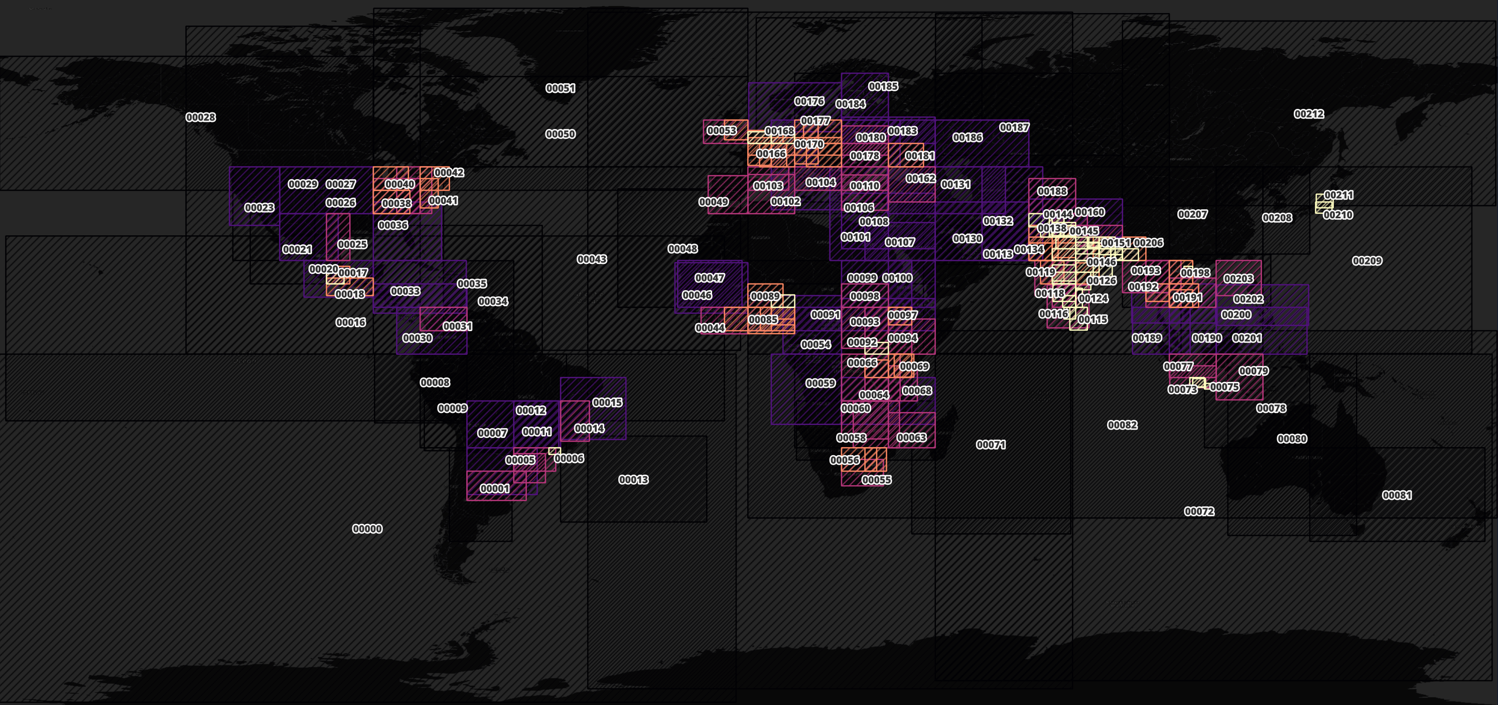
The 213 Parquet files containing building footprints are spatially sorted. Though any Parquet file's extents can overlap one or more other files, a city's buildings can often be found in just one or two Parquet files. Below is a map of where each Parquet file's extents cover.
$ ~/duckdb
COPY (
    SELECT SPLIT_PART(filename, '-', 2) as pq_num,
           {min_x: MIN(bbox.xmin),
            min_y: MIN(bbox.ymin),
            max_x: MAX(bbox.xmax),
            max_y: MAX(bbox.ymax)}::BOX_2D::GEOMETRY AS geom,
           ST_AREA(geom) AS area
    FROM READ_PARQUET('*.parquet', filename=true)
    GROUP BY filename
) TO 'pq_bboxes.gpkg'
        WITH (FORMAT GDAL,
              DRIVER 'GPKG',
              LAYER_CREATION_OPTIONS 'WRITE_BBOX=YES');
If I look for files that cover a single point I can get numerous results.
SELECT   *
FROM     ST_READ('pq_bboxes.gpkg')
WHERE    ST_CONTAINS(geom, ST_POINT(15.457, 49.446))
ORDER BY area;
┌─────────┬──────────────────────┬──────────────────────────────────────────────────────────────────────────────────────────────────┐
│  files  │         area         │                                               geom                                               │
│ varchar │        double        │                                             geometry                                             │
├─────────┼──────────────────────┼──────────────────────────────────────────────────────────────────────────────────────────────────┤
│ 00171   │  2.769453431842703e… │ POLYGON ((11.249471664428711 45.702972412109375, 11.249471664428711 50.625492095947266, 16.875…  │
│ 00172   │  4.7468249449466386… │ POLYGON ((14.062142372131348 44.99976348876953, 14.062142372131348 50.62534713745117, 22.50006…  │
│ 00173   │  4.7472419363330116… │ POLYGON ((11.249390602111816 47.812171936035156, 11.249390602111816 52.031532287597656, 22.500…  │
│ 00170   │  0.00012656948977713 │ POLYGON ((5.625179767608643 44.999698638916016, 5.625179767608643 56.250404357910156, 16.87509…  │
│ 00177   │  0.0003797018767757… │ POLYGON ((11.249753952026367 44.99969482421875, 11.249753952026367 67.50009155273438, 28.12509…  │
│ 00185   │  0.0019429114400682… │ POLYGON ((2.003997564315796 45.000179290771484, 2.003997564315796 80.81690216064453, 56.249927…  │
│ 00054   │ 0.018940577378506598 │ POLYGON ((-38.470733642578125 -80.41725158691406, -38.470733642578125 82.1736831665039, 78.021…  │
└─────────┴──────────────────────┴──────────────────────────────────────────────────────────────────────────────────────────────────┘
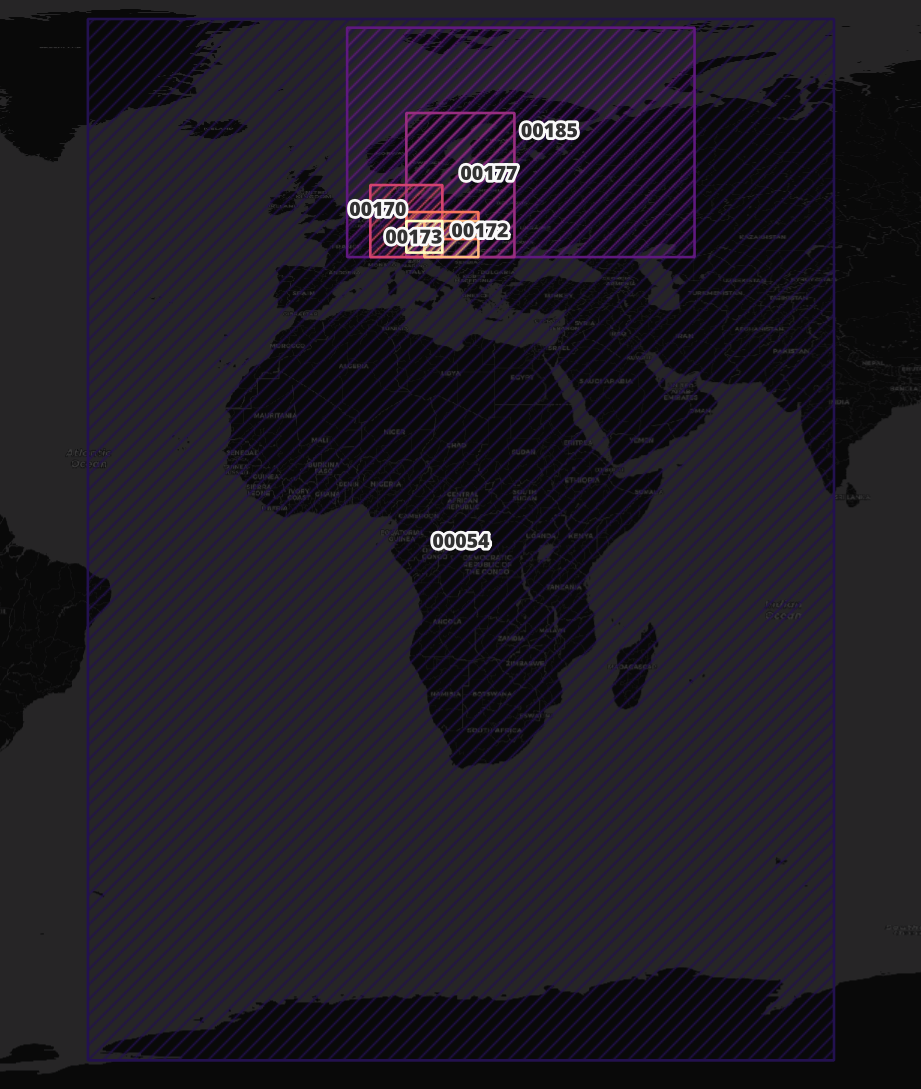
But if I search for an area instead, I can narrow the number of files of interest down considerably.
SELECT   DISTINCT filename
FROM     READ_PARQUET('*.parquet',
                      filename=True)
WHERE    ST_CONTAINS({min_x: 14.5519,   min_y: 50.1562,
                      max_x: 15.5619,   max_y: 49.2414}::BOX_2D,
                     {min_x: bbox.xmin, min_y: bbox.ymin,
                      max_x: bbox.xmax, max_y: bbox.ymax}::BOX_2D)
ORDER BY 1;
┌───────────────────────────────────────────────────────────────────┐
│                             filename                              │
│                              varchar                              │
├───────────────────────────────────────────────────────────────────┤
│ part-00171-ad3ba139-0181-4cec-a708-4d76675a32b0-c000.zstd.parquet │
│ part-00172-ad3ba139-0181-4cec-a708-4d76675a32b0-c000.zstd.parquet │
└───────────────────────────────────────────────────────────────────┘
I've found on my machine I can open any one building footprint Parquet file in QGIS and it will load reasonably quickly. The scene takes a second or two to refresh after every pan or zoom event.
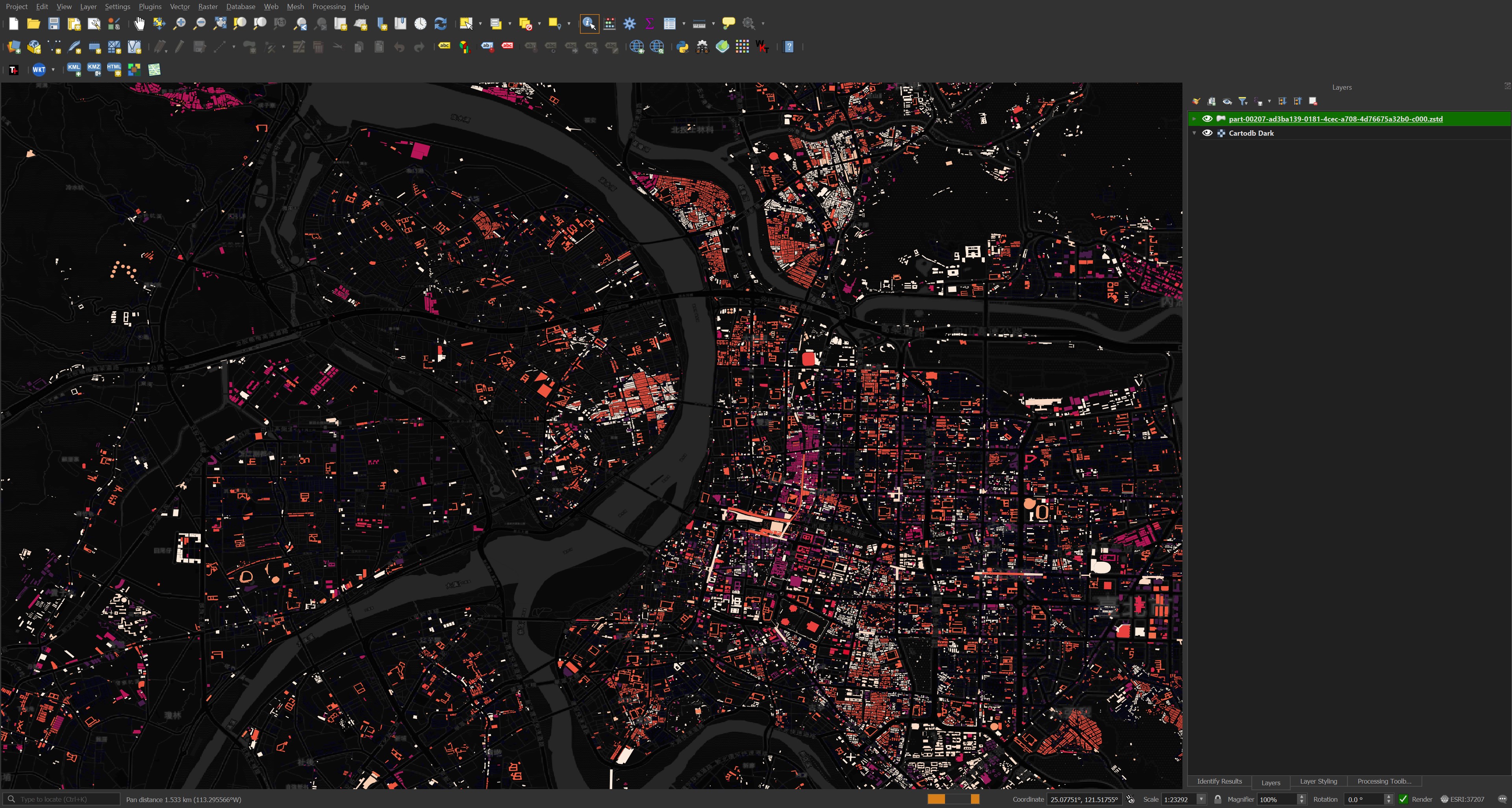
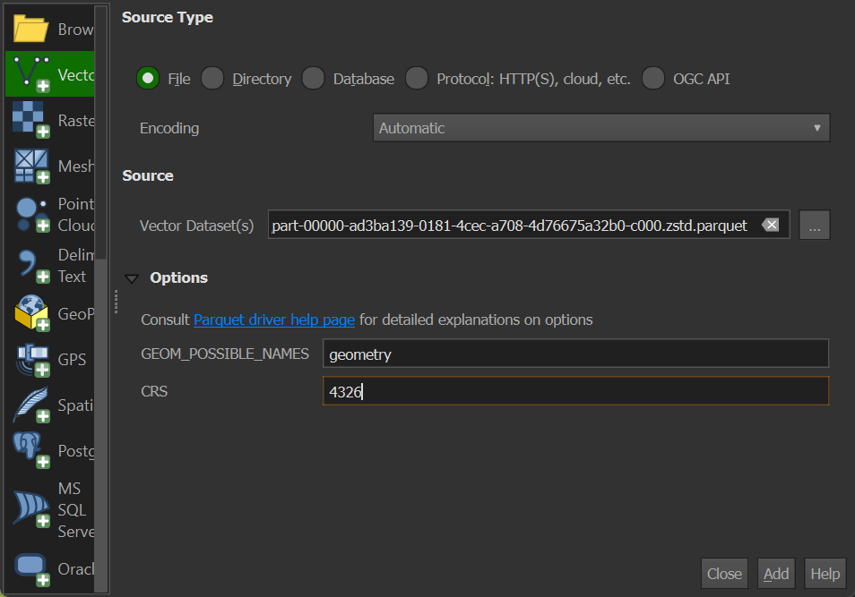
You can't just drag and drop Overture's Parquet files into a QGIS scene. Instead, you need to go to the Layer Menu -> Add Layer -> Add Vector Layer. Then in that dialog select your Parquet file of interest, set the geometry field name to "geometry" and set the projection to "4326".
Mapping to GeoFabrik
It's possible to find building footprints in this dataset based on locations used by GeoFabrik's OSM datasets. Below I'll download GeoFabrik's spatial partitions list.
$ wget -O geofabrik.geojson \
    https://download.geofabrik.de/index-v1.json
Below is an example record. I've excluded the geometry field for readability.
$ jq -S '.features[0]' geofabrik.geojson \
    | jq 'del(.geometry)'
{
  "properties": {
    "id": "afghanistan",
    "iso3166-1:alpha2": [
      "AF"
    ],
    "name": "Afghanistan",
    "parent": "asia",
    "urls": {
      "bz2": "https://download.geofabrik.de/asia/afghanistan-latest.osm.bz2",
      "history": "https://osm-internal.download.geofabrik.de/asia/afghanistan-internal.osh.pbf",
      "pbf": "https://download.geofabrik.de/asia/afghanistan-latest.osm.pbf",
      "pbf-internal": "https://osm-internal.download.geofabrik.de/asia/afghanistan-latest-internal.osm.pbf",
      "shp": "https://download.geofabrik.de/asia/afghanistan-latest-free.shp.zip",
      "taginfo": "https://taginfo.geofabrik.de/asia:afghanistan",
      "updates": "https://download.geofabrik.de/asia/afghanistan-updates"
    }
  },
  "type": "Feature"
}
These records cover anywhere with a landmass on Earth.
I'll import GeoFabrik's spatial partitions into DuckDB.
$ ~/duckdb
CREATE OR REPLACE TABLE geofabrik AS
    SELECT * EXCLUDE(urls),
           REPLACE(urls::JSON->'$.pbf', '"', '') AS url
    FROM ST_READ('geofabrik.geojson');
Below I'll list out all of the files containing the OSM data for Monaco.
SELECT   id, url
FROM     geofabrik
WHERE    ST_CONTAINS(geom, ST_POINT(7.4210967, 43.7340769))
ORDER BY ST_AREA(geom);
┌────────────────────────────┬───────────────────────────────────────────────────────────────────────────────────────┐
│             id             │                                          url                                          │
│          varchar           │                                        varchar                                        │
├────────────────────────────┼───────────────────────────────────────────────────────────────────────────────────────┤
│ monaco                     │ https://download.geofabrik.de/europe/monaco-latest.osm.pbf                            │
│ provence-alpes-cote-d-azur │ https://download.geofabrik.de/europe/france/provence-alpes-cote-d-azur-latest.osm.pbf │
│ alps                       │ https://download.geofabrik.de/europe/alps-latest.osm.pbf                              │
│ france                     │ https://download.geofabrik.de/europe/france-latest.osm.pbf                            │
│ europe                     │ https://download.geofabrik.de/europe-latest.osm.pbf                                   │
└────────────────────────────┴───────────────────────────────────────────────────────────────────────────────────────┘
Some areas have more than one file covering their geometry. This allows for downloading smaller files if you're only interested in a certain location or a larger file if you want to explore a larger area. Western Europe is heavily partitioned as shown below.
I'll load in the bounding boxes for each of Overture's building footprints and join them with GeoFabrik's partitions.
CREATE OR REPLACE TABLE overture AS
    SELECT   *
    FROM     ST_READ('pq_bboxes.gpkg');

CREATE OR REPLACE TABLE osm_overture AS
    SELECT DISTINCT a.id    AS osm_id,
                    b.files AS ov_buildings
    FROM geofabrik a
    JOIN overture b ON ST_INTERSECTS(a.geom, b.geom);
Now I can look up which Overture files contain data for Asia.
SELECT   ov_buildings
FROM     osm_overture
WHERE    osm_id = 'asia'
ORDER BY 1;
┌──────────────┐
│ ov_buildings │
│   varchar    │
├──────────────┤
│ 00028        │
│ 00054        │
│ 00071        │
│ 00072        │
│ 00073        │
│ 00074        │
│ 00075        │
│ 00076        │
│ 00077        │
│ 00078        │
│ 00079        │
│ 00080        │
│ 00082        │
│ 00097        │
│ 00099        │
│ 00100        │
├──────────────┤
│   16 rows    │
└──────────────┘
Asian Building Data
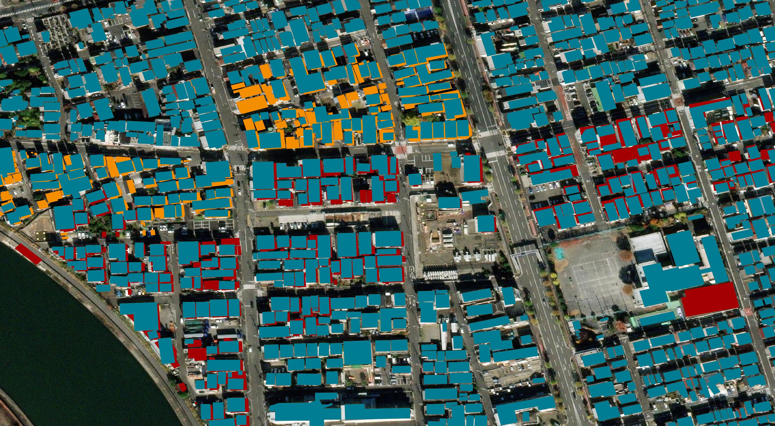
Within any one city change is constant. The following shows buildings in central Tokyo in blue that were in the April dataset. Orange are the changes from the June release and red are the changes from this month's release.
Unfortunately, between Vietnam and Japan, the building coverage drops off dramatically compared to everywhere else in the world.
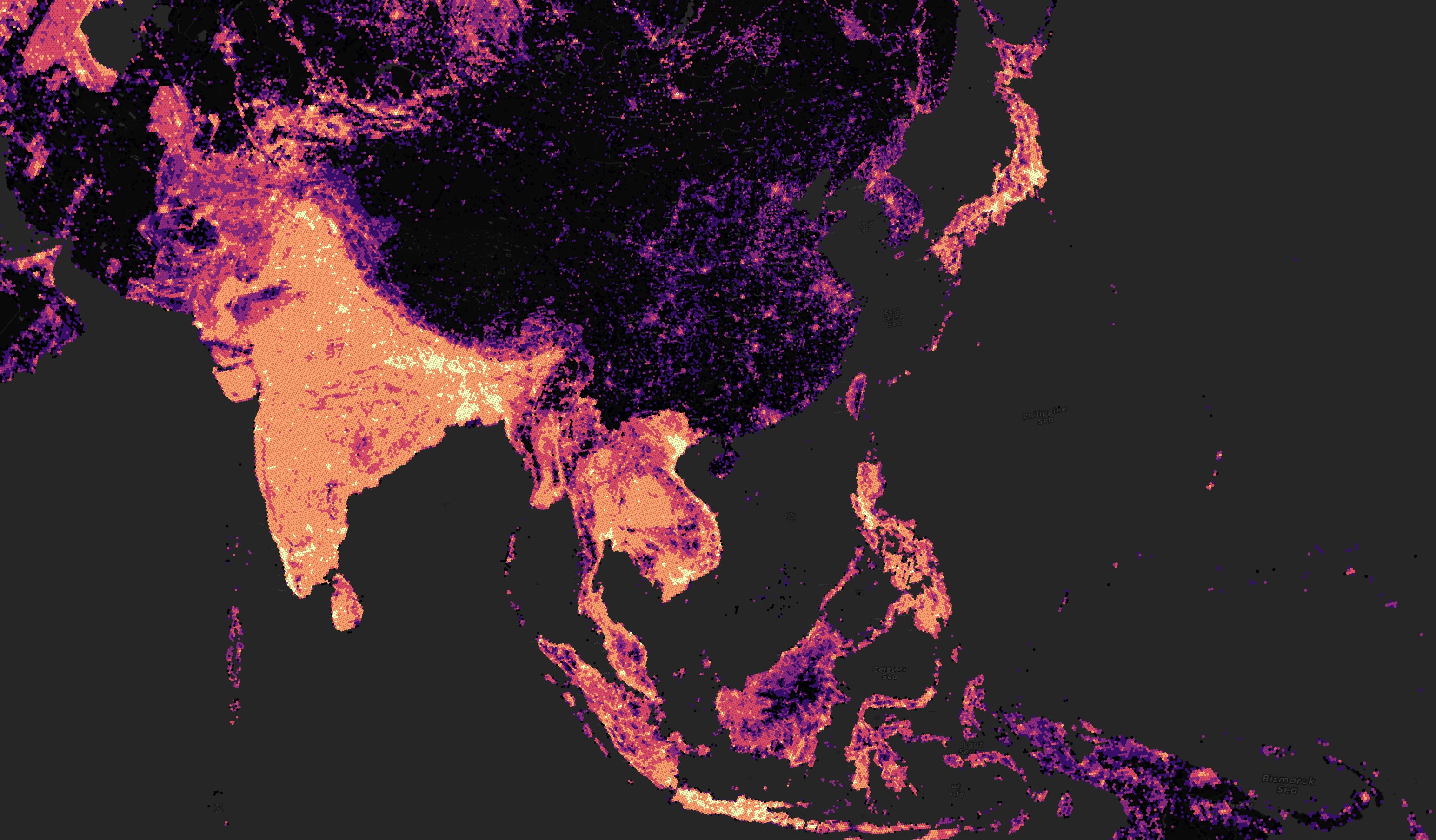
I don't have a good alternative for building footprint data in this part of the world at the moment but I recently reviewed a dataset produced via AI which aimed to help detect building footprints in several countries in Eastern Asia. There are some impressive results but the problem is far from solved.
Asian Mega-Cities
I wanted to get an idea of the state of Overture's building footprint coverage across major Asian Capitals. Below I built bounding boxes around 32 cities that Natural Earth says is both a political capital and a "mega-city" in Asia.
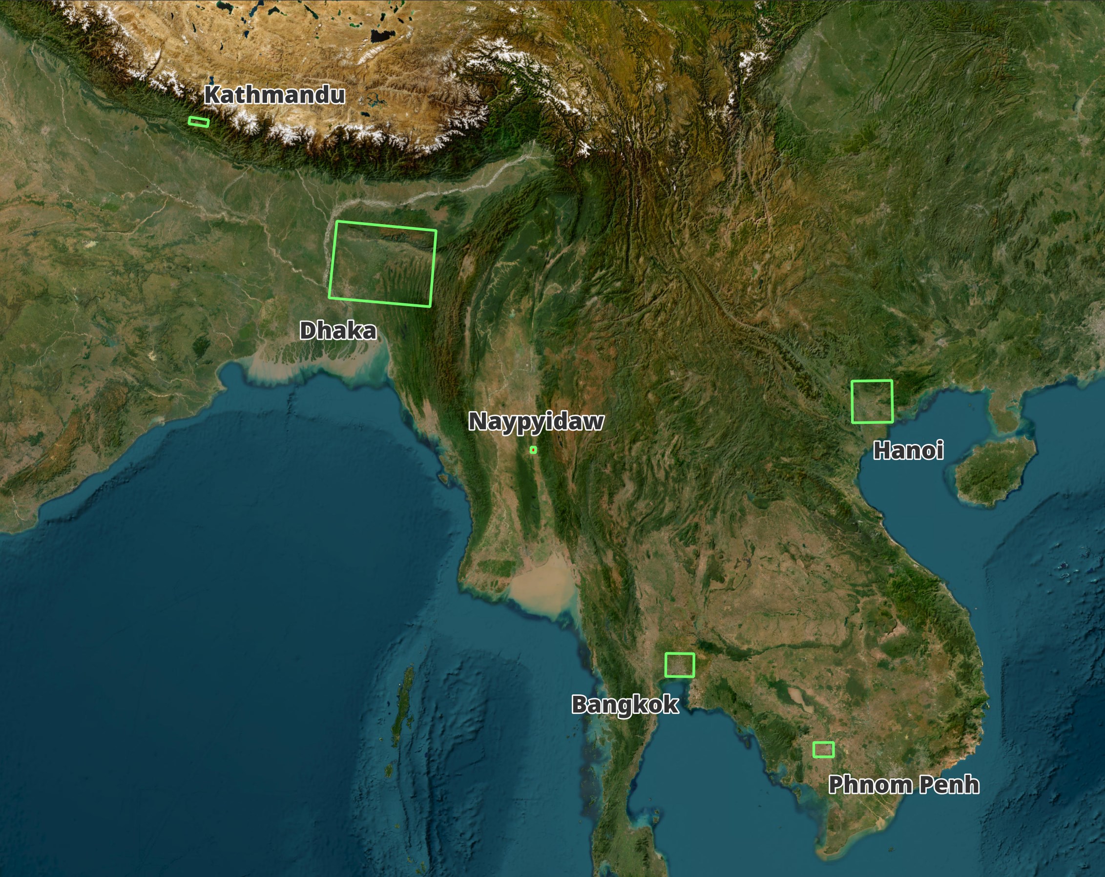
Most of the bounding boxes are pretty good but none are perfect. Some cut right through the middle of the cities I'm attempting to analyse while others overextend into neighbouring states.
I then used the bounding boxes to extract each city's building footprints from Overture into their own GPKG files.
$ cd ~/2024_07/theme\=buildings/type\=building
$ python3
import json

import duckdb
from   rich.progress import track


sql_bboxes = '''
    CREATE OR REPLACE TABLE city_bboxes AS
        SELECT a.NAME_EN,
               a.ADM0CAP::BOOL  AS is_capital,
               a.MEGACITY::BOOL AS is_mega_city,
               b.CONTINENT      AS continent,
               {min_x: a.MAX_BBXMIN,
                min_y: a.MAX_BBYMIN,
                max_x: a.MAX_BBXMAX,
                max_y: a.MAX_BBYMAX }::BOX_2D::GEOMETRY AS bbox_max
        FROM ST_READ('/home/mark/natural_earth/10m_cultural/ne_10m_populated_places/ne_10m_populated_places.shx') a
        JOIN ST_READ('/home/mark/natural_earth/10m_cultural/ne_10m_admin_0_countries/ne_10m_admin_0_countries.shx') b
                ON a.ADM0_A3 = b.ISO_A3
        WHERE a.MAX_BBXMIN
        AND   a.MAX_BBYMIN
        AND   a.MAX_BBXMAX
        AND   a.MAX_BBYMAX
        AND   (a.ADM0CAP OR a.MEGACITY);'''

sql_asian_mega_cities = '''
    SELECT   NAME_EN           AS city_name,
             ST_XMIN(bbox_max) AS xmin,
             ST_XMAX(bbox_max) AS xmax,
             ST_YMIN(bbox_max) AS ymin,
             ST_YMAX(bbox_max) AS ymax,
    FROM     city_bboxes
    WHERE    continent = 'Asia'
    AND      is_capital
    AND      is_mega_city
    ORDER BY ST_AREA(bbox_max);'''

sql_export = '''
    COPY (
        SELECT a.id                                 AS id,
               a.version                            AS version,
               a.subtype                            AS subtype,
               a.class                              AS class,
               a.level                              AS level,
               a.has_parts                          AS has_parts,
               a.height                             AS height,
               a.is_underground                     AS is_underground,
               a.num_floors                         AS num_floors,
               a.num_floors_underground             AS num_floors_underground,
               a.min_height                         AS min_height,
               a.min_floor                          AS min_floor,
               a.facade_color                       AS facade_color,
               a.facade_material                    AS facade_material,
               a.roof_material                      AS roof_material,
               a.roof_shape                         AS roof_shape,
               a.roof_direction                     AS roof_direction,
               a.roof_orientation                   AS roof_orientation,
               a.roof_color                         AS roof_color,
               a.roof_height                        AS roof_height,
               JSON(a.names)                        AS names,
               JSON(a.bbox)                         AS bbox,
               JSON(a.sources)                      AS sources,
               ST_GeomFromWKB(a.geometry)::GEOMETRY AS geom
        FROM   READ_PARQUET('*.parquet') a
        WHERE  bbox.xmin > ?
        AND    bbox.xmax < ?
        AND    bbox.ymin > ?
        AND    bbox.ymax < ?
    ) TO '%s'
        WITH (FORMAT GDAL,
              DRIVER 'GPKG',
              LAYER_CREATION_OPTIONS 'WRITE_BBOX=YES');'''

con = duckdb.connect(database=':memory:')

for ext in ('spatial', 'parquet'):
    con.sql('INSTALL %s; LOAD %s;' % (ext, ext))

con.sql(sql_bboxes)
df = con.sql(sql_asian_mega_cities).to_df()

for rec in track(list(df.iloc())):
    try:
        con.sql(sql_export % ('%s.gpkg' % rec.city_name,),
                params=(rec.xmin,
                        rec.xmax,
                        rec.ymin,
                        rec.ymax))
    except Exception as exc:
        print(exc)
I can see 10s of MB/s of data being read and written when the above is being executed. I haven't yet found a way to make the most of my 24-core CPU during this process though.
At best, two cores are maxed out. There are 100s of parquet files being read so I suspect this is a workload that could be scaled across the other cores better.
The above produced an 885 MB GPKG file for Islamabad, Pakistan in three hours. This works out to an average of 34 MB/s of Parquet data being read and ~85 KB/s of GPKG data being written.
I revisited the export performance of GPKG versus Parquet after my initial publication of this post and I found Parquet to generate ~300x faster than GPKG.
Islamabad's Building Footprints
The bounding box for Islamabad erroneously cut right through the middle of the city so the building counts below won't tell the whole story. That said, Google's Open Buildings dataset is the primary source of data followed by Microsoft with OSM coming in a distant third.
$ ~/duckdb
SELECT   sources->0->'dataset' AS source,
         COUNT(*)
FROM     ST_READ('Islamabad.gpkg')
GROUP BY 1
ORDER BY 2 DESC;
┌──────────────────────────┬──────────────┐
│          source          │ count_star() │
│           json           │    int64     │
├──────────────────────────┼──────────────┤
│ "Google Open Buildings"  │      1022149 │
│ "Microsoft ML Buildings" │       536444 │
│ "OpenStreetMap"          │         4840 │
└──────────────────────────┴──────────────┘
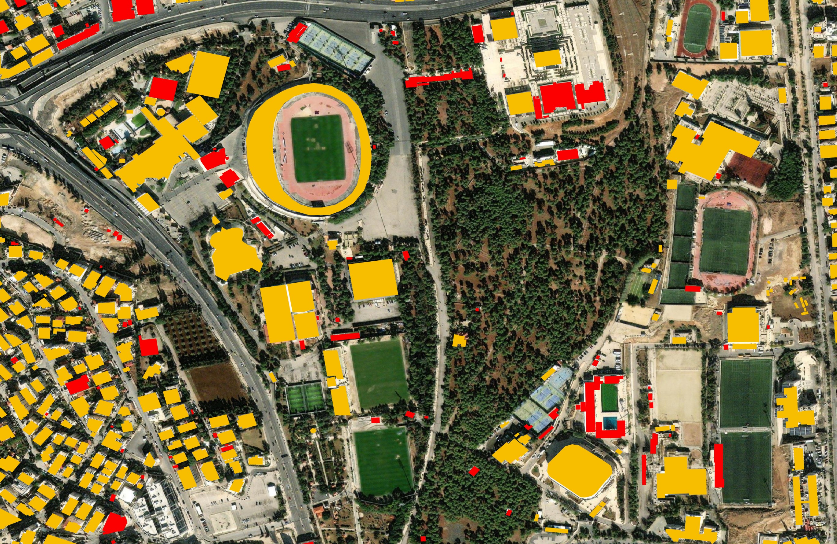
The buildings below are yellow for OSM, red for Microsoft and light-blue for Google.
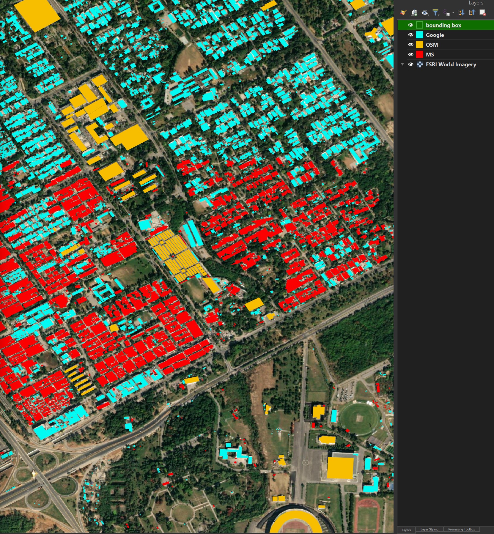
MS buildings can often have unnatural shapes. Overture doesn't seem to prefer OSM building data even though many exist in OSM. Given OSM demands human-verified building footprints and is the only source with rich metadata, I'm surprised they're not picked over Google and Microsoft.
Google's buildings seem to be made out of plausible rectangles and rarely have unnatural shapes.
The unnatural and more complex geometry Microsoft has produced can be seen in their average geometry field length compared to Google and OSM.
SELECT   sources->0->'dataset' AS source,
         AVG(LENGTH(geom))
FROM     ST_READ('Islamabad.gpkg')
GROUP BY 1
ORDER BY 2 DESC;
┌──────────────────────────┬────────────────────┐
│          source          │ avg(length(geom))  │
│           json           │       double       │
├──────────────────────────┼────────────────────┤
│ "Microsoft ML Buildings" │ 237.70458799054515 │
│ "Google Open Buildings"  │  197.4561546310763 │
│ "OpenStreetMap"          │  195.0685950413223 │
└──────────────────────────┴────────────────────┘
OSM often has decimal values for its vertices to the 7th decimal place, Google has to the 13th decimal place and Microsoft has to the 14th decimal place.
SELECT   sources->0->'dataset' AS source,
         AVG(LENGTH(SPLIT_PART(ST_XMIN(geom)::TEXT, '.', 2))) AS decimal_places
FROM     ST_READ('Islamabad.gpkg')
GROUP BY 1
ORDER BY 2 DESC;
┌──────────────────────────┬────────────────────┐
│          source          │   decimal_places   │
│           json           │       double       │
├──────────────────────────┼────────────────────┤
│ "Microsoft ML Buildings" │ 13.842589347629948 │
│ "Google Open Buildings"  │ 12.612874443941147 │
│ "OpenStreetMap"          │  6.887603305785124 │
└──────────────────────────┴────────────────────┘
Missing Building Metadata
As stated before, OSM is the only one of these three data sources that has rich metadata for buildings. Below you can see that ~10% of their building data for Islamabad has a floor count compared to none for Google or Microsoft.
$ ~/duckdb
WITH a AS (
    SELECT   sources->0->'dataset' AS source,
             num_floors IS NULL    AS has_floors,
             COUNT(*)                 cnt
    FROM     ST_READ('Islamabad.gpkg')
    GROUP BY 1, 2
)
PIVOT a
ON    has_floors
USING SUM(cnt);
┌──────────────────────────┬────────┬─────────┐
│          source          │ false  │  true   │
│           json           │ int128 │ int128  │
├──────────────────────────┼────────┼─────────┤
│ "OpenStreetMap"          │    438 │    4402 │
│ "Google Open Buildings"  │        │ 1022149 │
│ "Microsoft ML Buildings" │        │  536444 │
└──────────────────────────┴────────┴─────────┘
Almost 20% of OSM records have a name associated with each building.
WITH a AS (
    SELECT sources->0->'dataset' AS source,
           names IS NOT NULL     AS has_name,
           COUNT(*)                 cnt
    FROM ST_READ('Islamabad.gpkg')
    GROUP BY 1, 2
)
PIVOT a
ON    has_name
USING SUM(cnt);
┌──────────────────────────┬─────────┬────────┐
│          source          │  false  │  true  │
│           json           │ int128  │ int128 │
├──────────────────────────┼─────────┼────────┤
│ "Microsoft ML Buildings" │  536444 │        │
│ "Google Open Buildings"  │ 1022149 │        │
│ "OpenStreetMap"          │    4025 │    815 │
└──────────────────────────┴─────────┴────────┘
OSM has a rich set of classes for each building as well.
WITH a AS (
    SELECT   sources->0->'dataset' AS source,
             class,
             COUNT(*) cnt
    FROM     ST_READ('Islamabad.gpkg')
    GROUP BY 1, 2
)
PIVOT    a
ON       source
USING    SUM(cnt)
ORDER BY 4 DESC;
┌────────────────────┬─────────────────────────┬──────────────────────────┬─────────────────┐
│       class        │ "Google Open Buildings" │ "Microsoft ML Buildings" │ "OpenStreetMap" │
│      varchar       │         int128          │          int128          │     int128      │
├────────────────────┼─────────────────────────┼──────────────────────────┼─────────────────┤
│                    │                 1022149 │                   536444 │            3416 │
│ house              │                         │                          │             766 │
│ commercial         │                         │                          │             142 │
│ semidetached_house │                         │                          │              82 │
│ hut                │                         │                          │              69 │
│ apartments         │                         │                          │              47 │
│ school             │                         │                          │              45 │
│ residential        │                         │                          │              38 │
│ mosque             │                         │                          │              37 │
│ university         │                         │                          │              30 │
│ train_station      │                         │                          │              17 │
│ hospital           │                         │                          │              15 │
│ office             │                         │                          │              13 │
│ hangar             │                         │                          │              13 │
│ stadium            │                         │                          │              13 │
│ warehouse          │                         │                          │              12 │
│ industrial         │                         │                          │              10 │
│ garage             │                         │                          │               9 │
│ college            │                         │                          │               7 │
│ library            │                         │                          │               6 │
│ retail             │                         │                          │               6 │
│ carport            │                         │                          │               6 │
│ bunker             │                         │                          │               5 │
│ post_office        │                         │                          │               5 │
│ hotel              │                         │                          │               4 │
│ parking            │                         │                          │               4 │
│ farm               │                         │                          │               3 │
│ grandstand         │                         │                          │               3 │
│ farm_auxiliary     │                         │                          │               3 │
│ shed               │                         │                          │               3 │
│ public             │                         │                          │               2 │
│ barn               │                         │                          │               2 │
│ government         │                         │                          │               2 │
│ detached           │                         │                          │               2 │
│ garages            │                         │                          │               1 │
│ transportation     │                         │                          │               1 │
│ church             │                         │                          │               1 │
├────────────────────┴─────────────────────────┴──────────────────────────┴─────────────────┤
│ 37 rows                                                                         4 columns │
└───────────────────────────────────────────────────────────────────────────────────────────┘
This building metadata could be a useful source of ground truth for Google and Microsoft.
Amman's Building Footprints
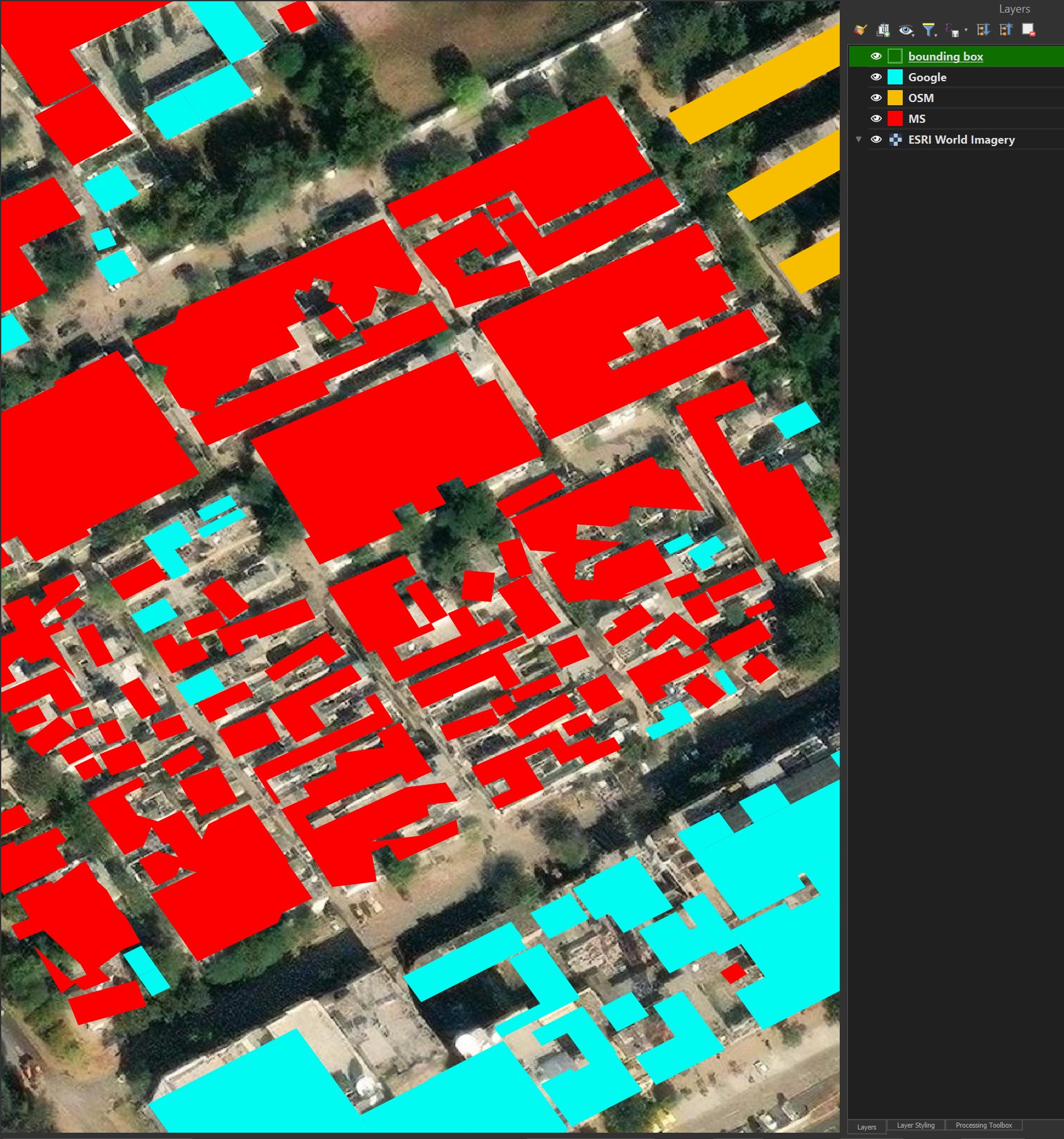
Amman, Jordan's dataset doesn't source any data from Google but does use Microsoft for the majority of its building footprints.
$ ~/duckdb
SELECT   sources->0->'dataset' AS source,
         COUNT(*)
FROM     ST_READ('Amman.gpkg')
GROUP BY 1
ORDER BY 2 DESC;
┌──────────────────────────┬──────────────┐
│          source          │ count_star() │
│           json           │    int64     │
├──────────────────────────┼──────────────┤
│ "Microsoft ML Buildings" │       333276 │
│ "OpenStreetMap"          │        79851 │
└──────────────────────────┴──────────────┘
Most buildings in the city are identified with only a few exceptions. There are a few examples where Microsoft couldn't detect a building, even if it was next to other similar-looking buildings.
A stone factory next to the Airport seems to have confused Microsoft's AI.
Buildings with walls between them are shown as being attached when they aren't.
The buildings in an auto parts yard look to be well-marked. This looks like it would be difficult to train AI for so I'm impressed with the results.
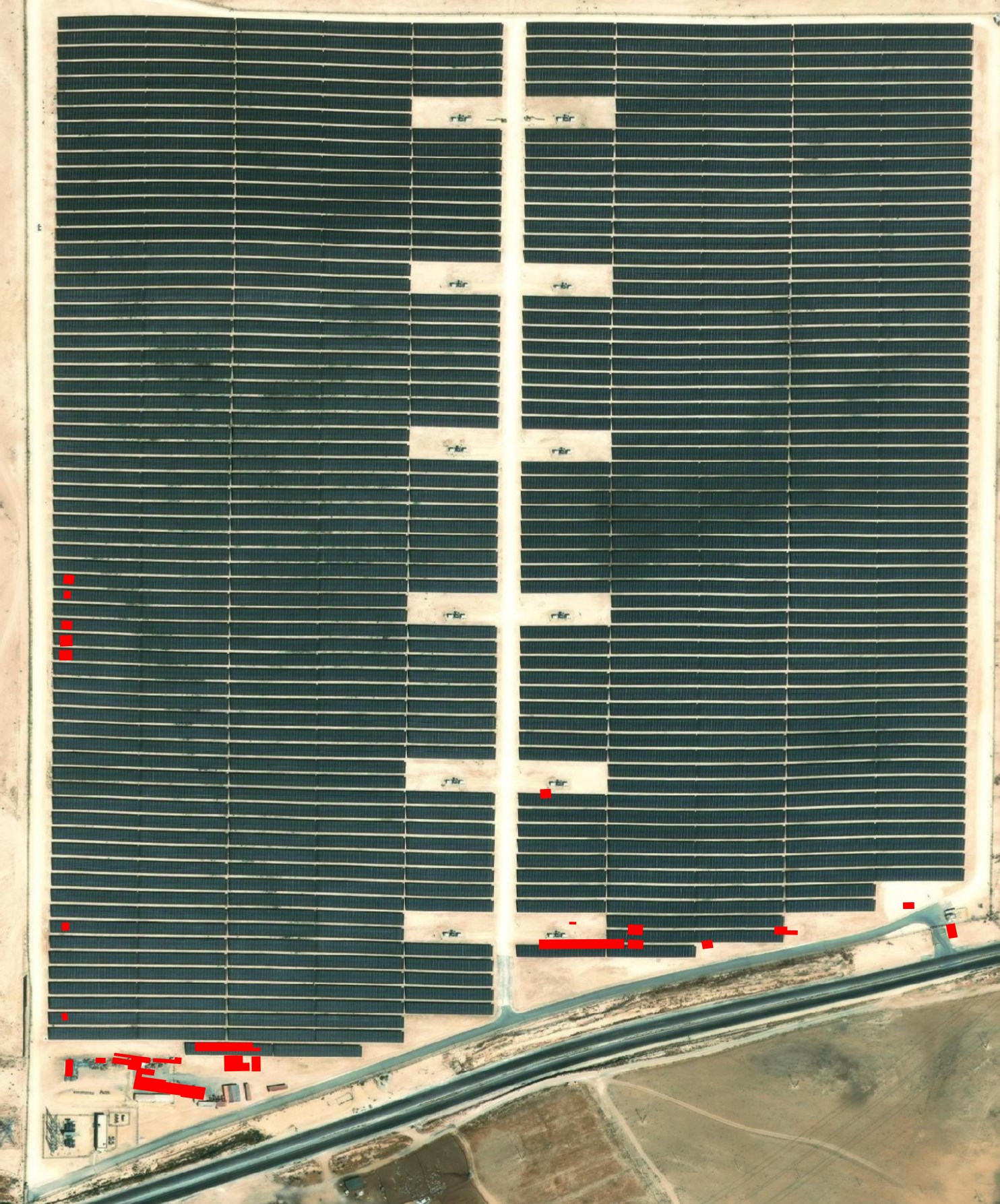
For the most part, large solar arrays aren't mistaken for buildings.
Sports pitches aren't mistaken for buildings. This is a step up from other building footprint detection AI models I've seen.
This solar park is almost perfect but has a few small, erroneous building footprints.
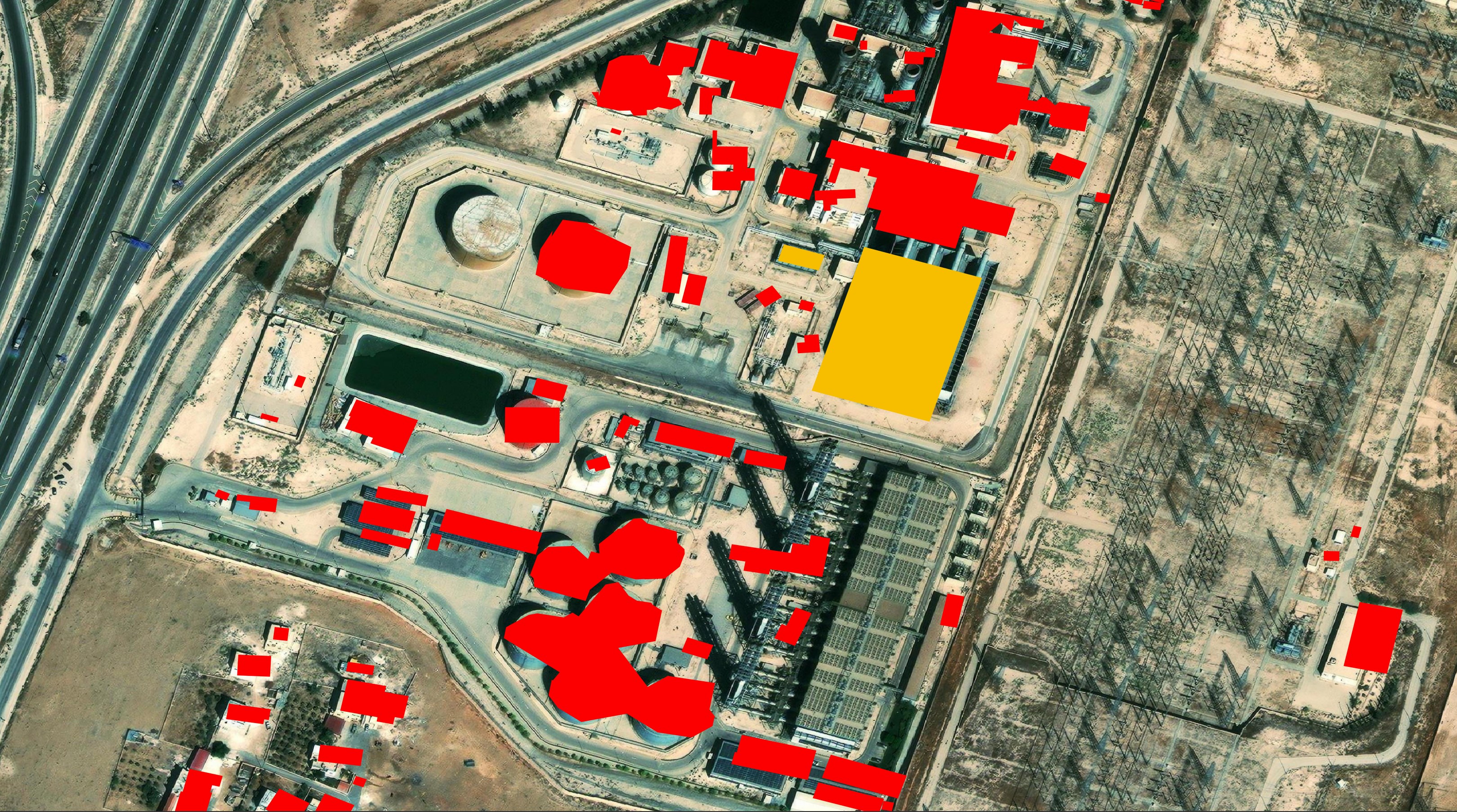
A few containers at this power generation facility are marked erroneous as buildings.
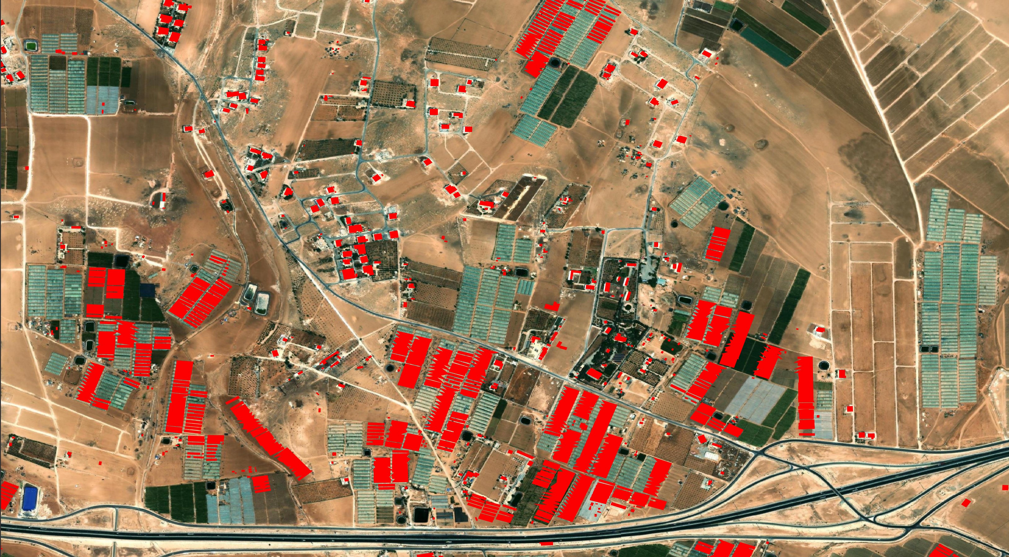
Some greenhouses are marked as buildings, others aren't.
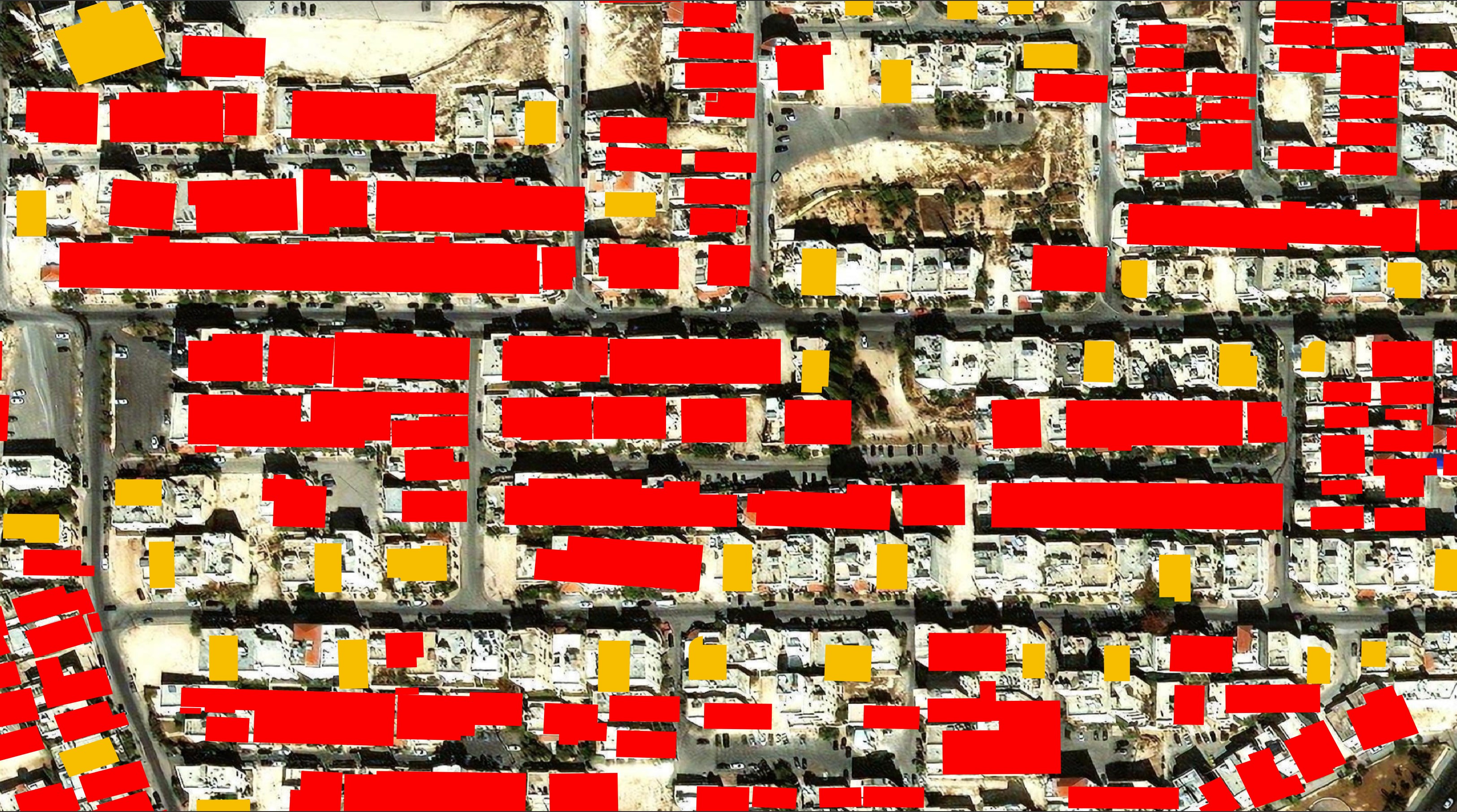
Ankara's Building Footprints
Microsoft and OSM have almost an equal number of building footprints for Ankara's dataset.
$ ~/duckdb
SELECT   sources->0->'dataset' AS source,
         COUNT(*)
FROM     ST_READ('Ankara.gpkg')
GROUP BY 1
ORDER BY 2 DESC;
┌──────────────────────────┬──────────────┐
│          source          │ count_star() │
│           json           │    int64     │
├──────────────────────────┼──────────────┤
│ "Microsoft ML Buildings" │       141914 │
│ "OpenStreetMap"          │       134532 │
└──────────────────────────┴──────────────┘
There are some buildings erroneously marked on highways and in the Airport's aircraft parking areas.
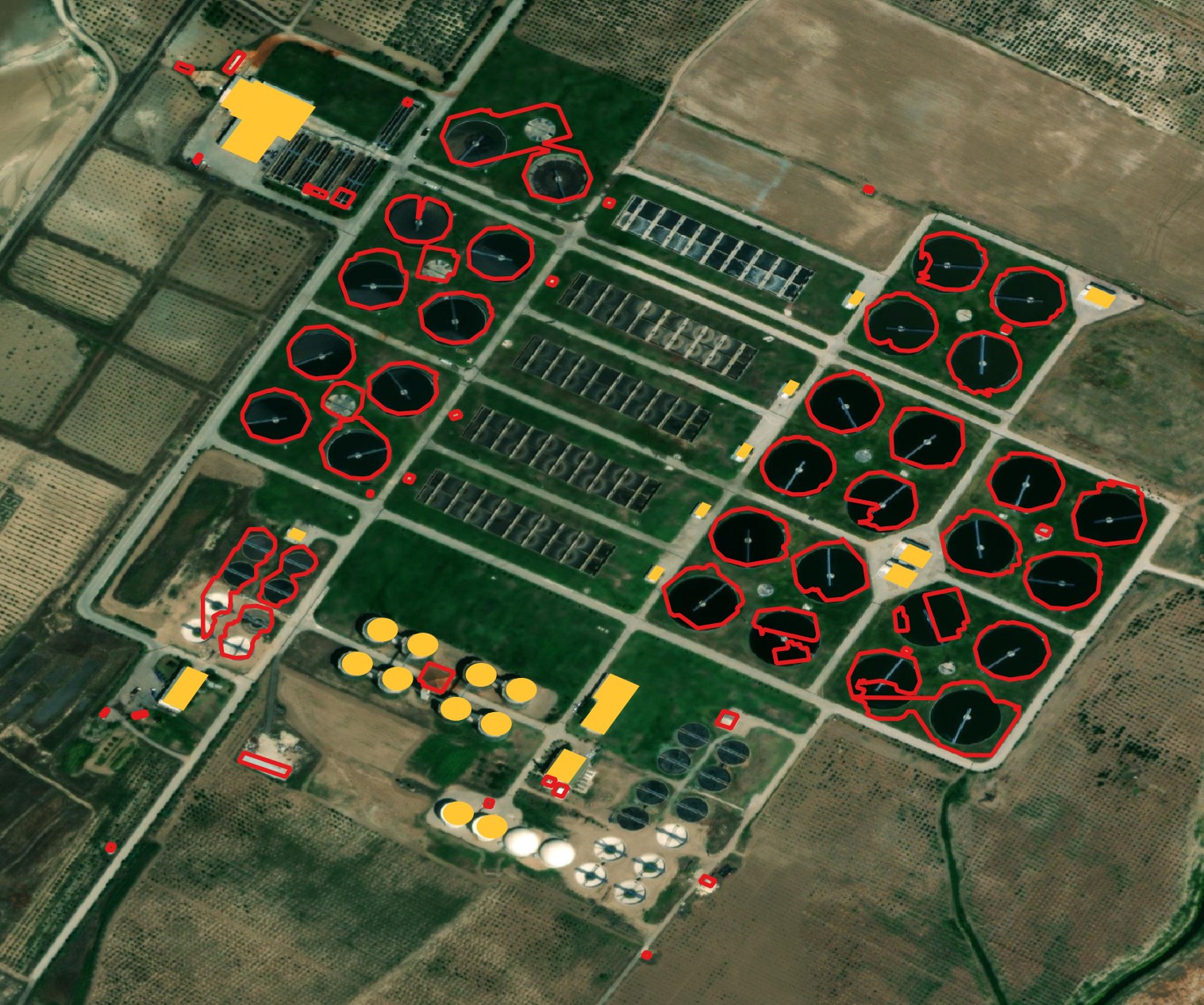
Some sewage treatment infrastructure has been erroneously marked as buildings.
Microsoft vs Google vs OSM
Google, Microsoft and OSM are the three data providers I'm seeing time and time again in Overture's Asian building footprints dataset.
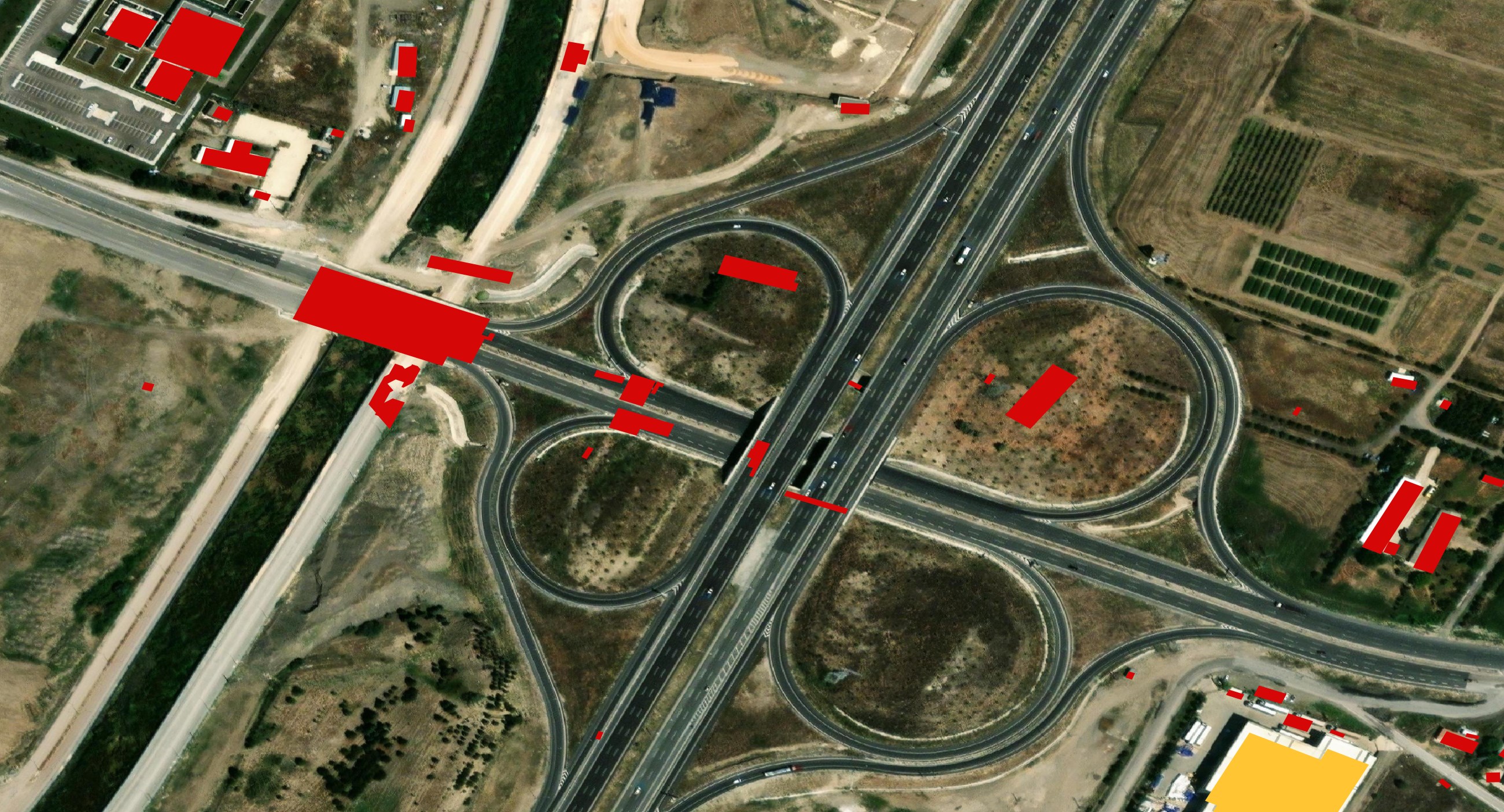
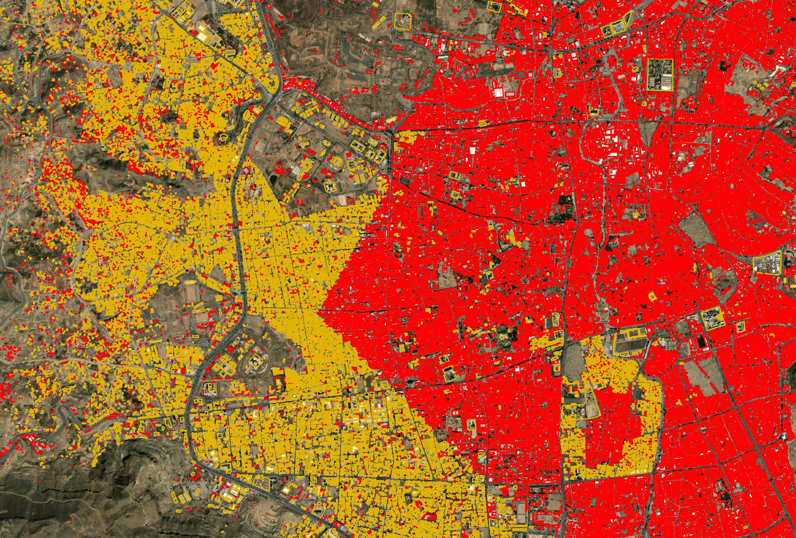
Below is in Baghdad. There are synthetic divisions where OSM data was preferred over what is mostly Microsoft geometry. I still can't see any clear pattern as to why one provider is picked over the other two in any of these cities I've looked at.
There is a tilted rectangle delineating areas where Microsoft's building footprints are preferred over OSM's in Sanaa, Yemen.
Priority for OSM Data
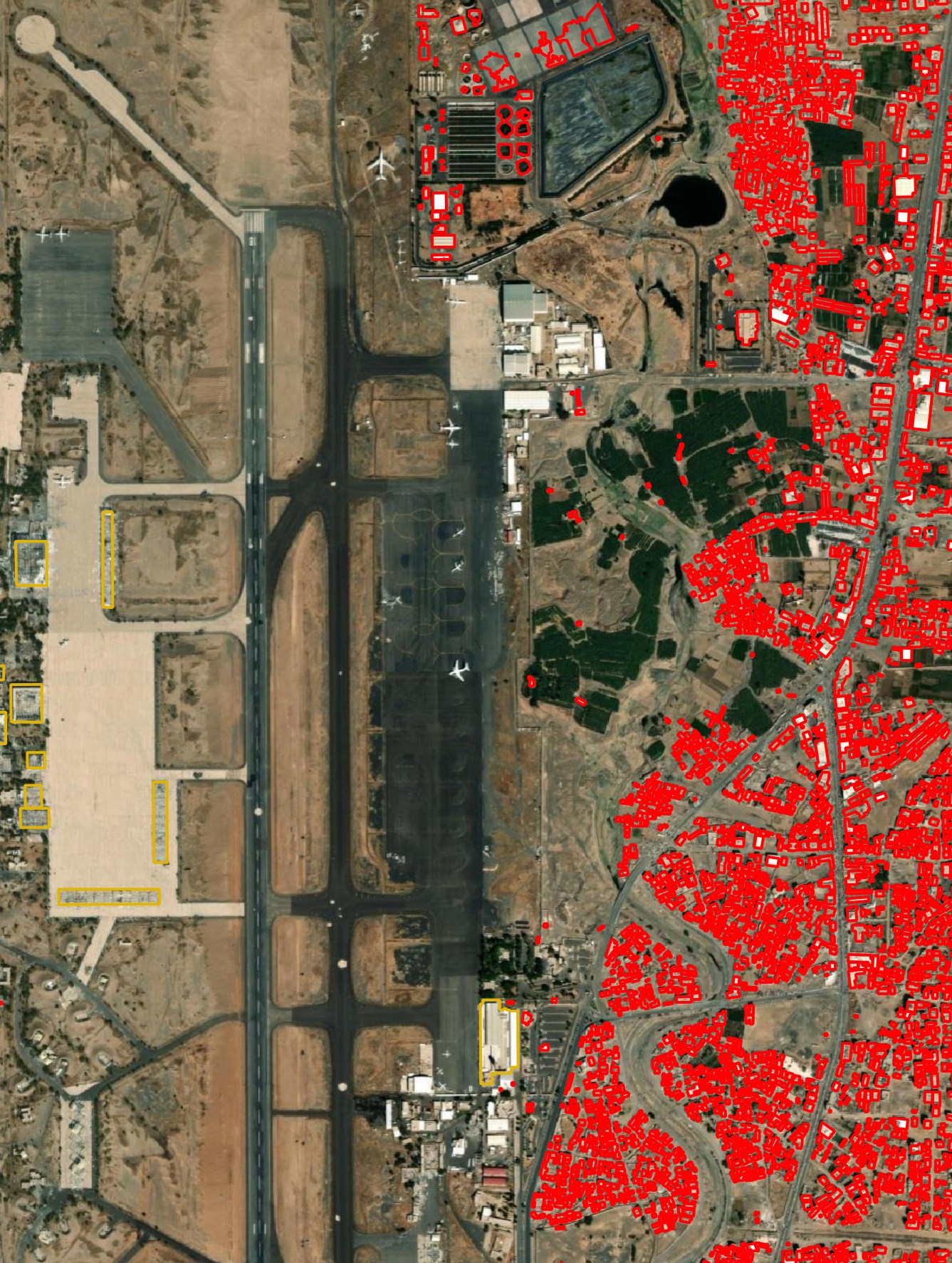
Microsoft's detections seem to suffer more than the other two providers in detecting buildings that aren't in any imagery I can source. The area surrounding the Uppatasanti Pagoda in Naypyidaw, Myanmar threw off Microsoft's AI.
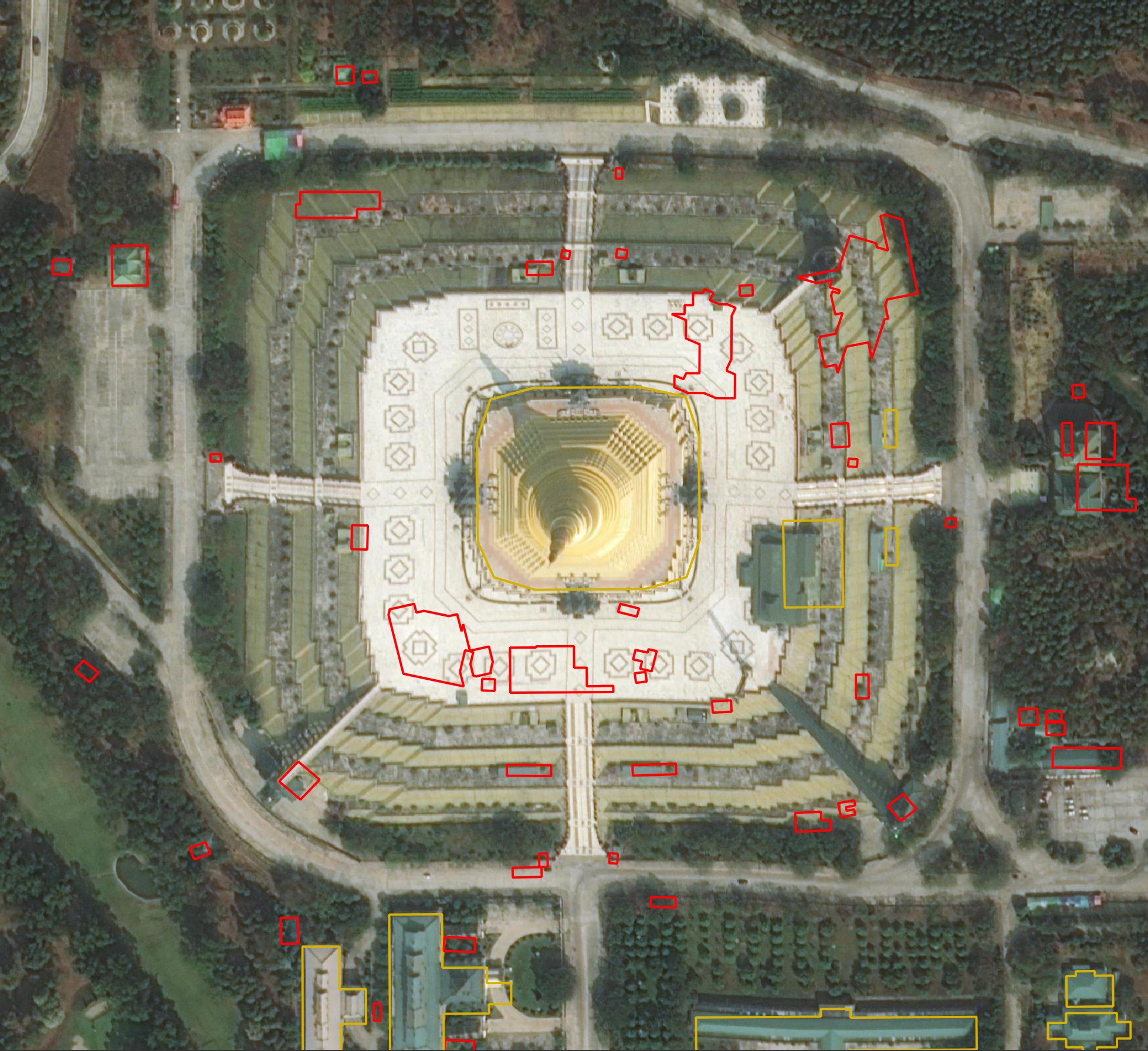
Below are several buildings Microsoft detected in Myanmar. I can't find any imagery of this area that shows these buildings being here.
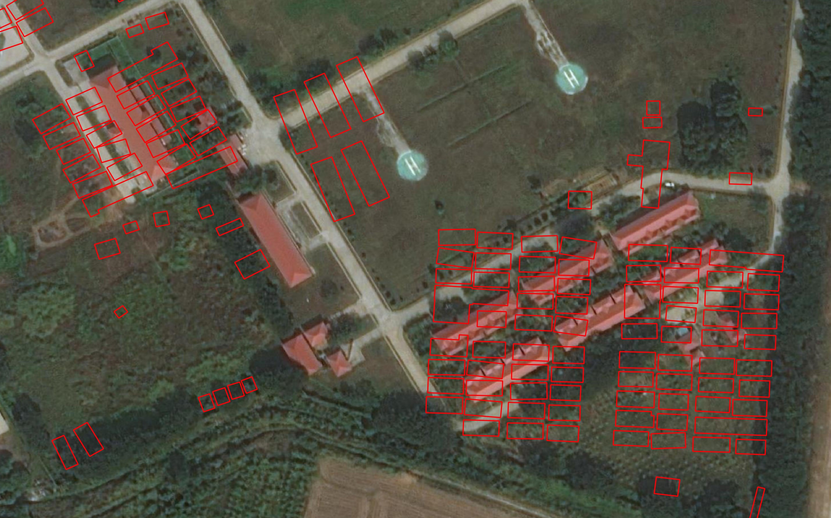
Microsoft detected a bunch of buildings in the middle of the river in Bangkok.
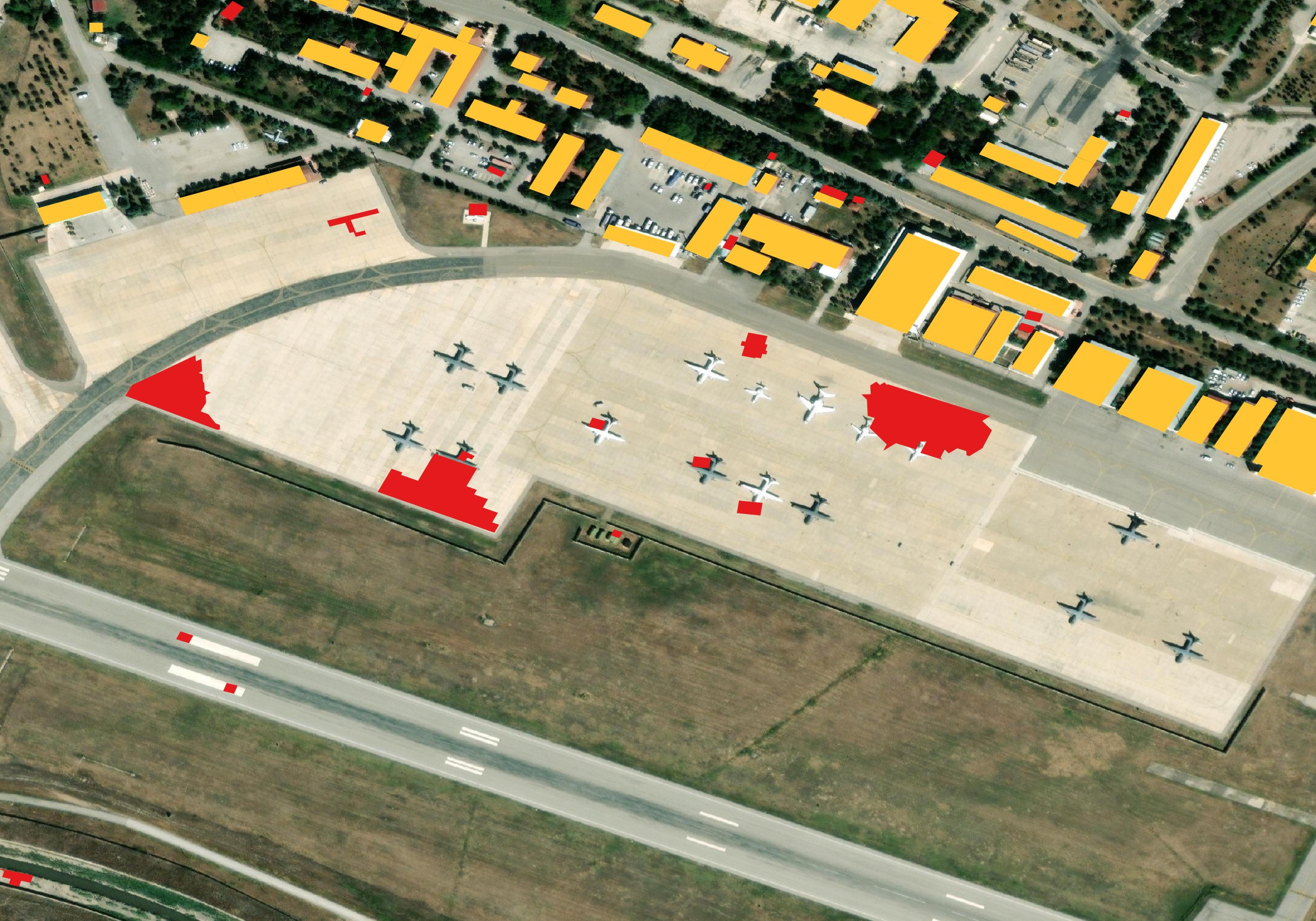
Microsoft detected buildings that don't exist in the parking lot at Beirut Airport.
There are also examples where detections are completely absent in an area surrounded by Microsoft detections. Very few of the buildings around Sanaa's airport are marked.
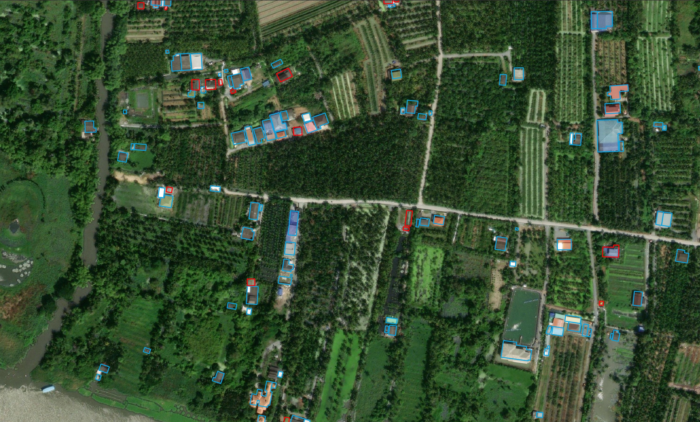
Google did a very good job of detecting buildings in the Thai countryside outside of Bangkok.
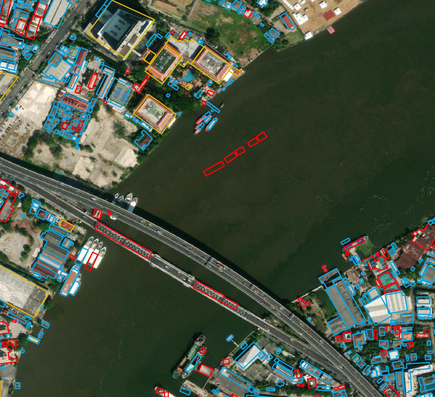
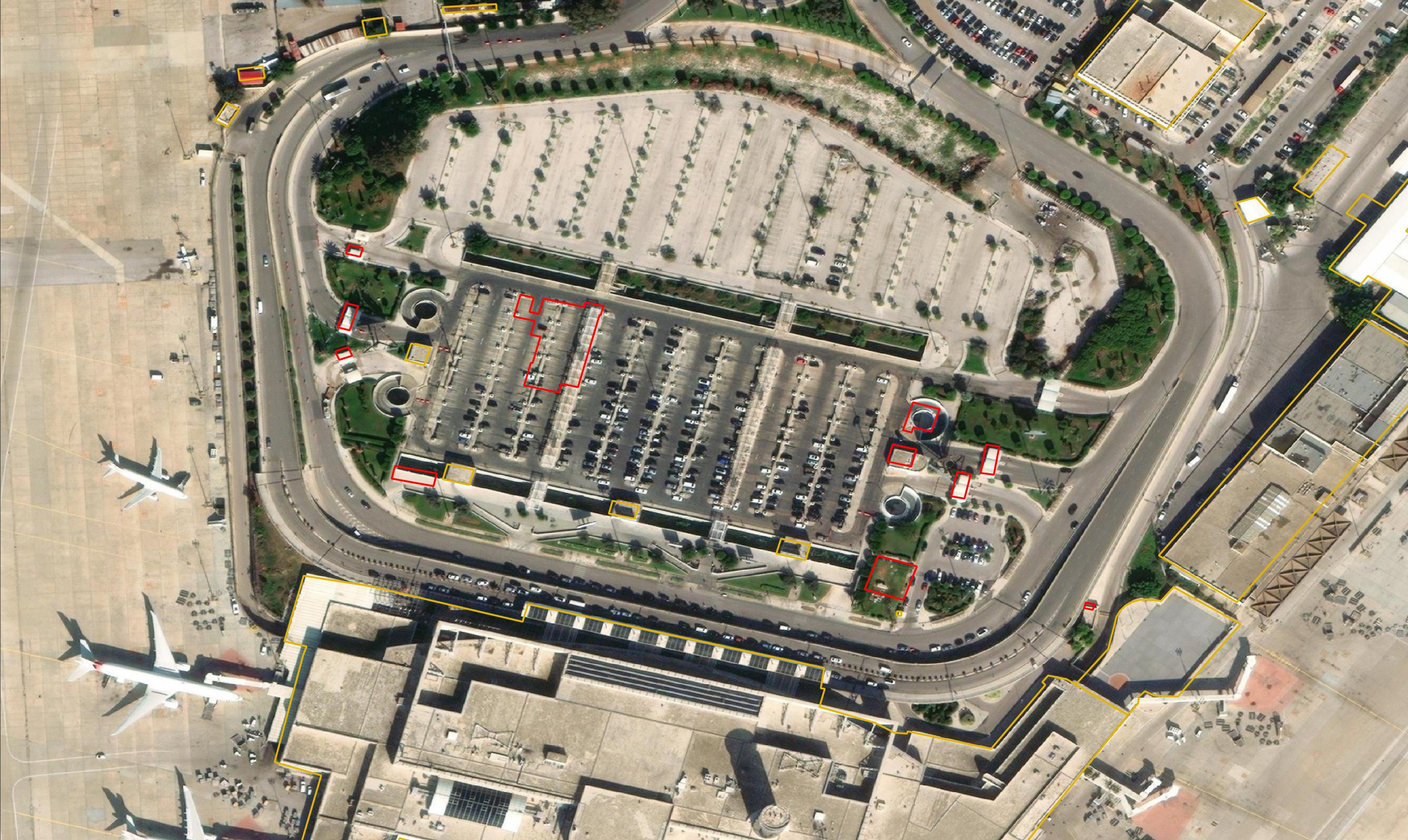
But Google also made some strange building predictions at Bangkok's Suvarnabhumi Airport (BKK).
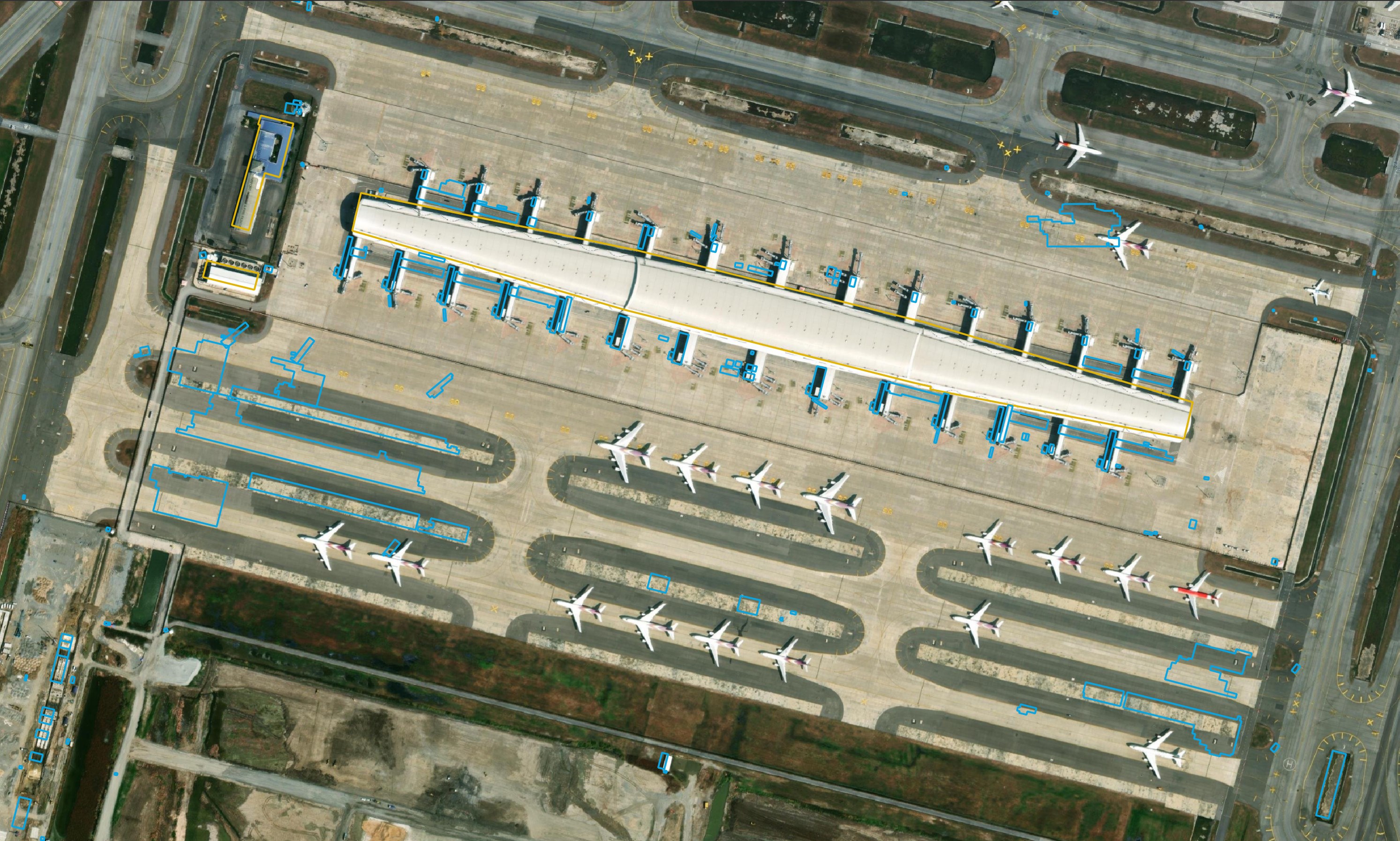
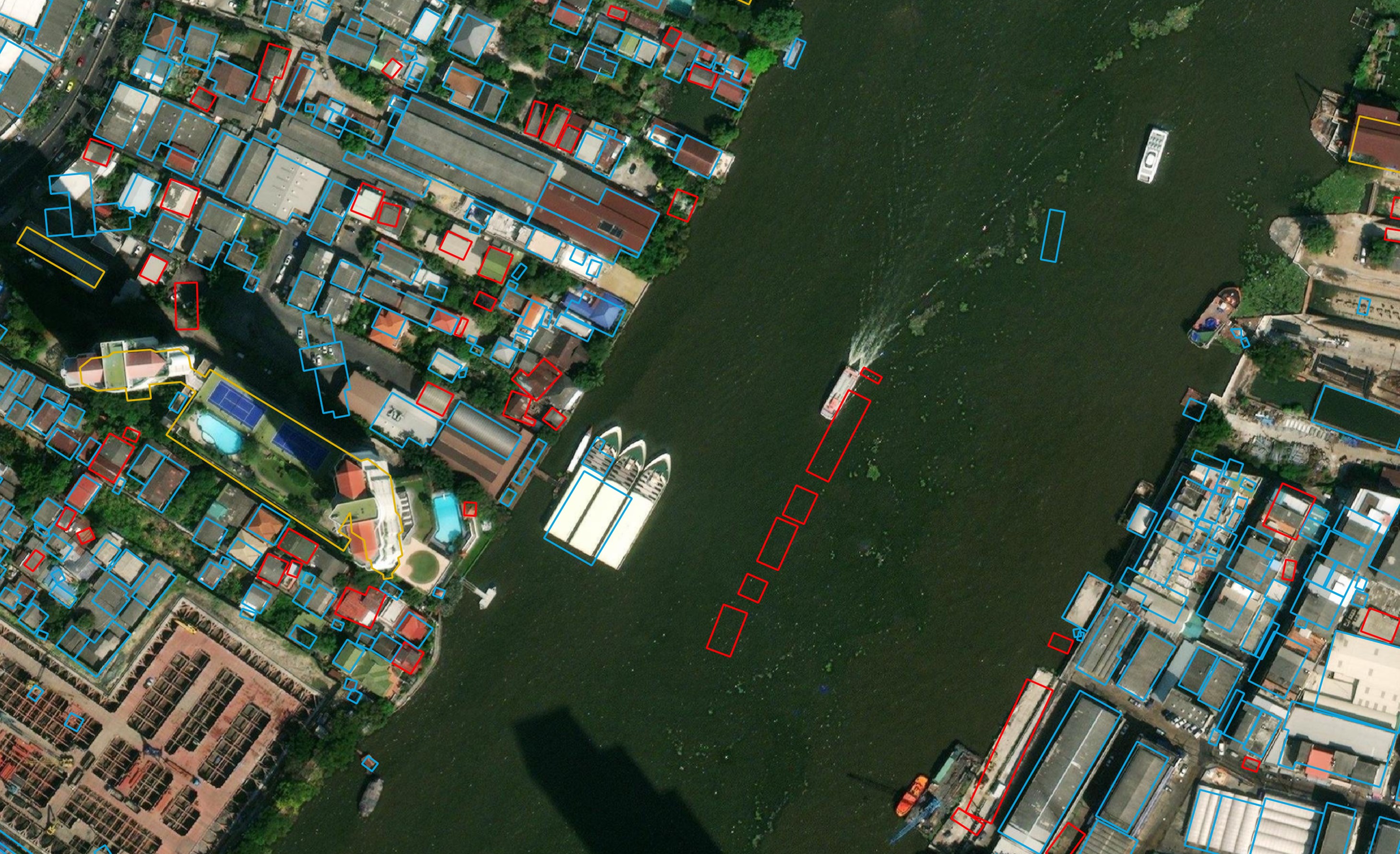
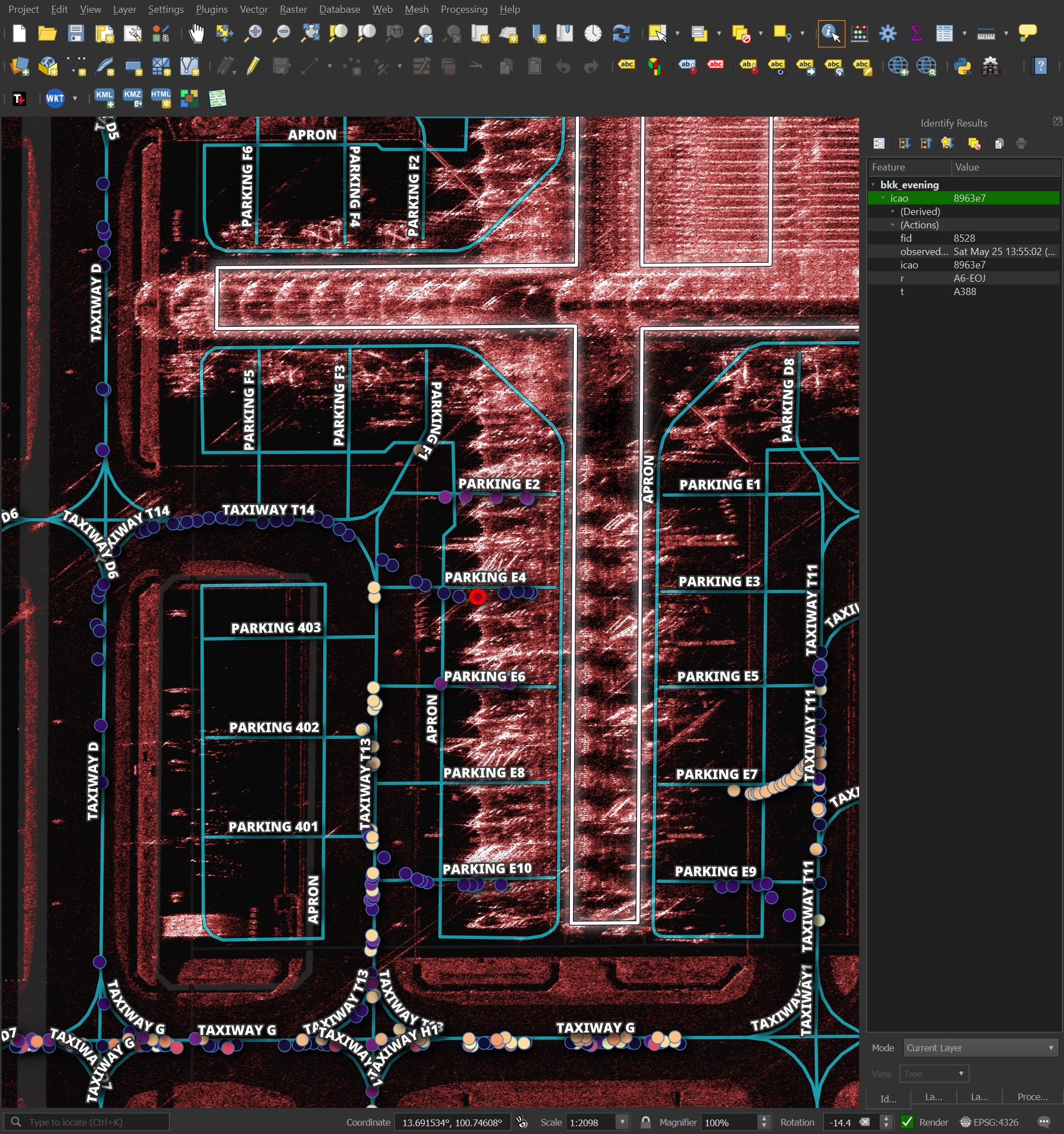
I've been looking closely at BKK's OSM data for an aircraft detection in SAR imagery project. The underlying pink-tinted imagery below is from Umbra. Excluding the dots of the aircraft positions, the geometry and label data is all from OSM.
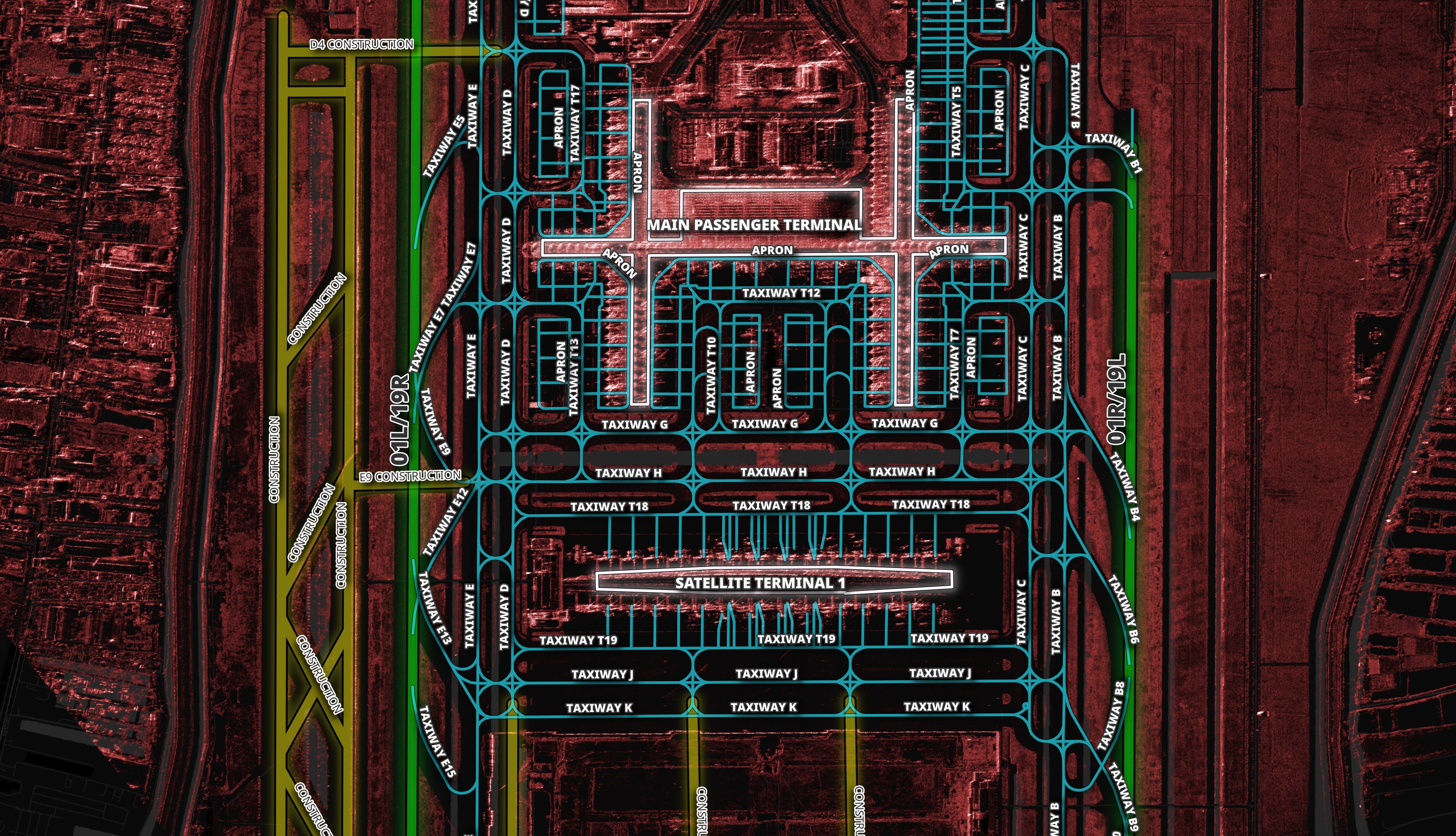
The geometry and metadata are as great as I could ever ask for. Below is a closer look at the aircraft parking bays. The OSM volunteers took their time to get this right.
Sam Chui flew from Qatar to Bangkok earlier this year and one of the pilots showed him the app they use to get runway and taxi information. The details on the screen aren't that much more detailed than what is available on OSM.
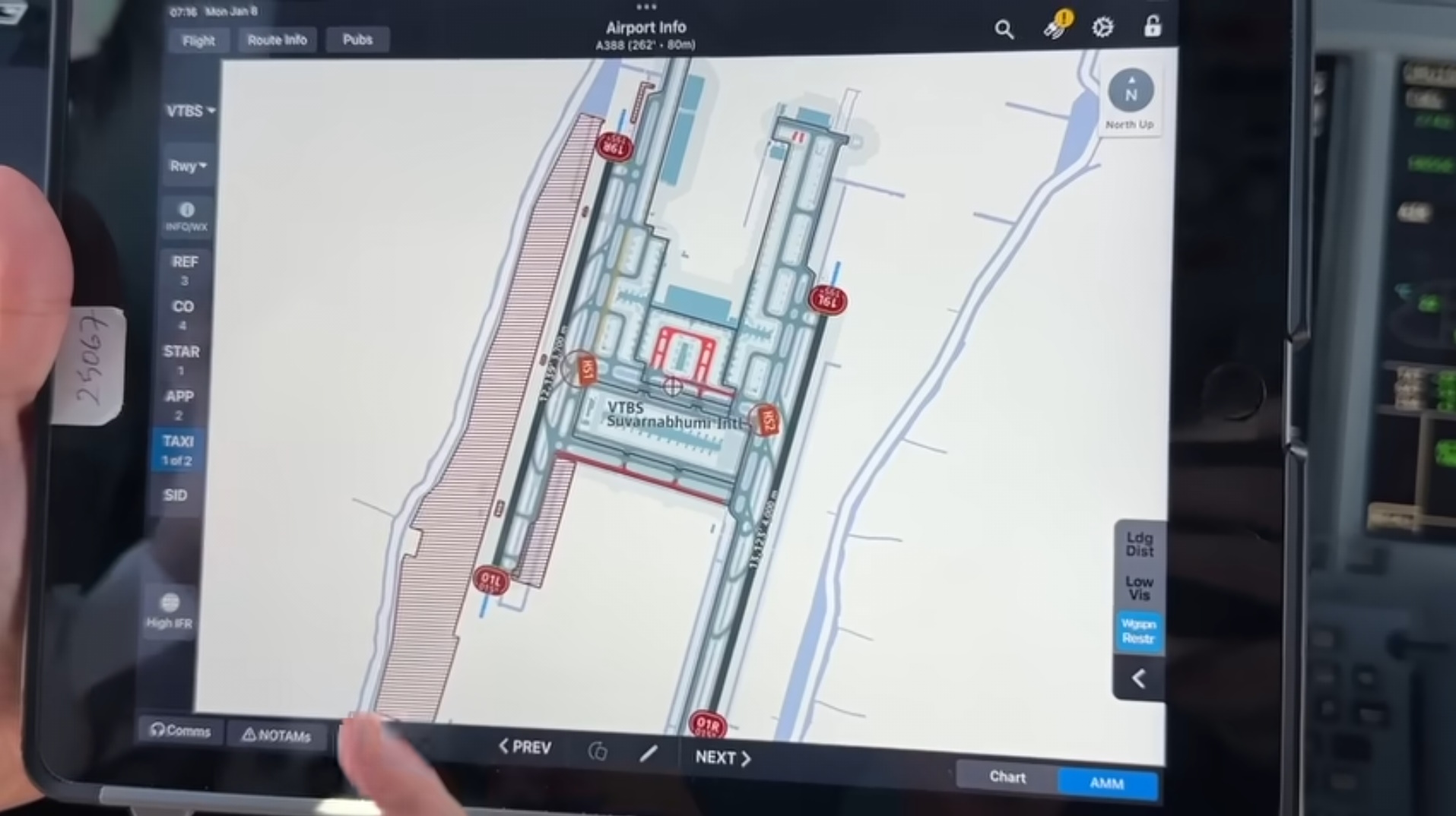


I suspect their data source has more people paid to make sure everything is very accurate but OSM is still a fantastic first source of GIS data.
If I were Overture, I would have geo-fenced major Airports with a high OSM data density and made sure these areas picked OSM data first.
When to opt for AI
There should be a stronger system to suspect when OSM data isn't as detailed as it could be. There is a textile factory in the middle of Sanaa where OSM has a single ~350 x 262-meter rectangle around the compound rather than the individual buildings.
This ended up being picked over Microsoft's building detection attempt. I feel that for buildings beyond a certain plausible size, Microsoft would make a better prediction.
AI Could Fill a Void
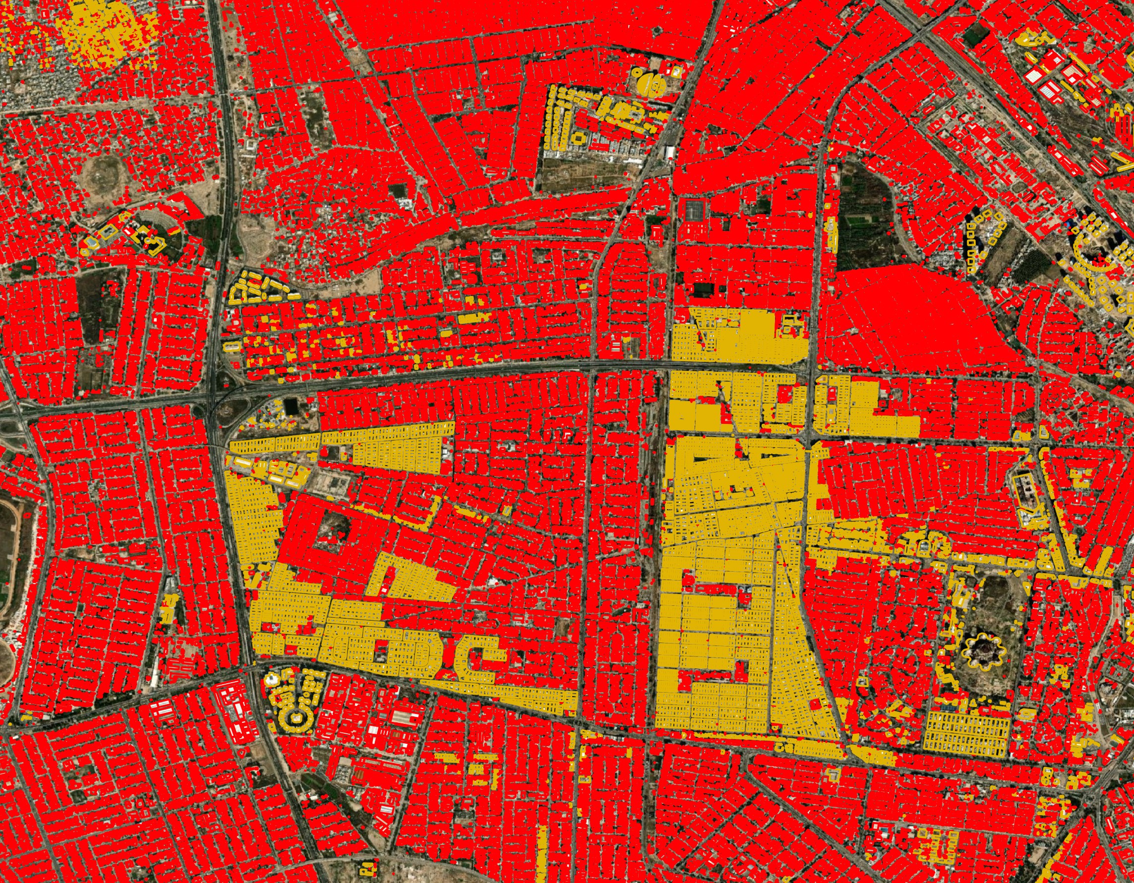
In Tbilisi, there are clusters of buildings where floor counts and other metadata are well-populated on OSM. But these are outliers and much of the city doesn't have much metadata at all. This same pattern can be found in many cities around the world.
OSM demands human-verified data. OSM has ~50K individuals contributing every month which is an incredible volunteer workforce. But even a workforce of this size hasn't been able to blanket every building in the world with rich metadata. AI is probably the only hope at this point if open and rich metadata describing buildings everywhere in the world is to be made available.