Maxar operates a fleet of satellites that capture imagery of the Earth. Some of these satellites offered the best resolution commercially available when they were first launched into space. In 2022, Maxar earned ~$1.6B largely from selling imagery these satellites produced.
Last year, they launched a Basemap service which offers 30cm resolution covering all of Earth's landmasses. This basemap was produced from 400K individual strips captured from their fleet of satellites. They mostly use imagery from recent springs and summers and have worked to produce imagery that looks seamless over large areas. The cities I'll look at in this post have less than 1% cloud cover and some are completely cloudless.
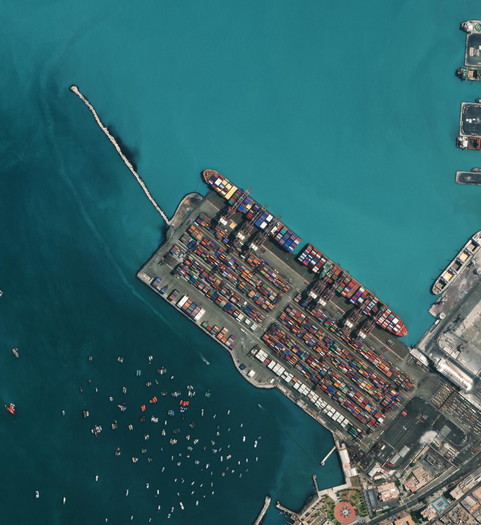
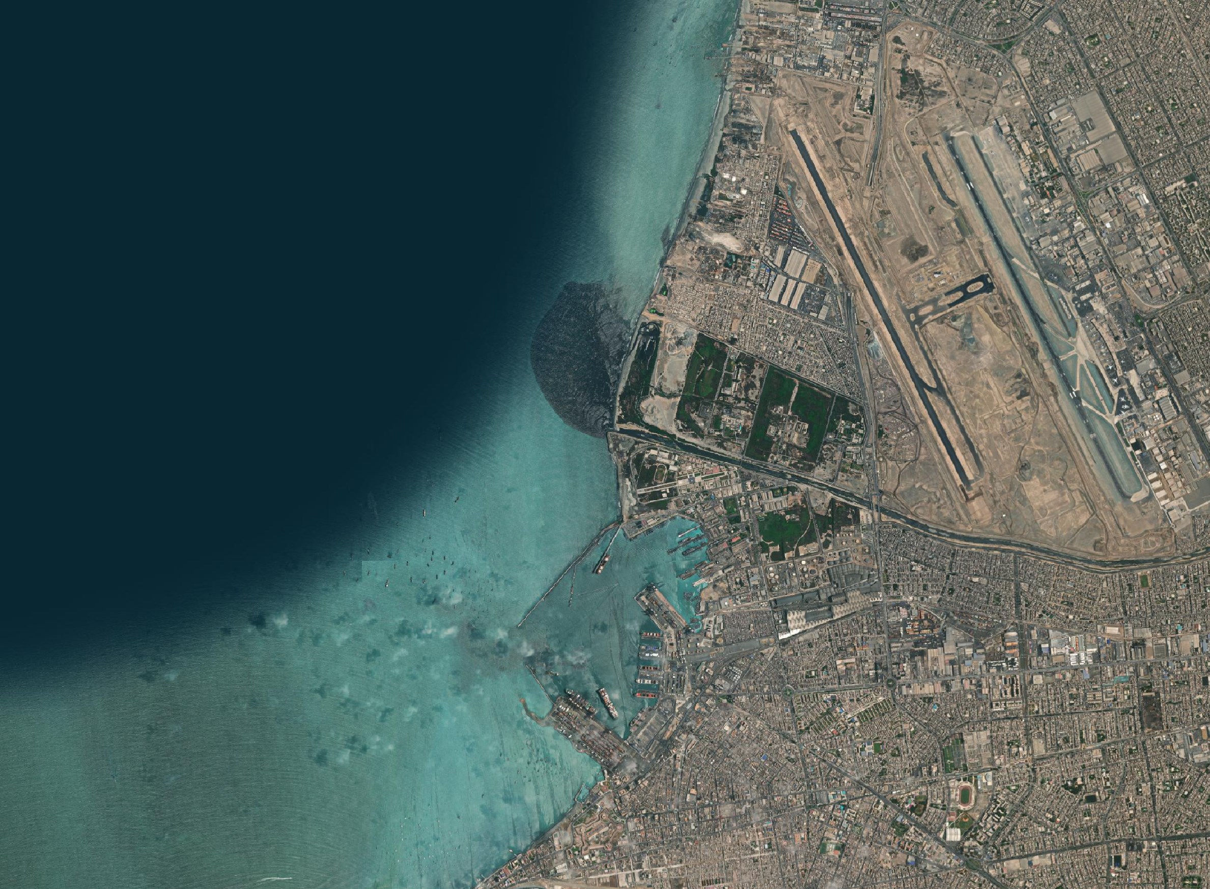
Below is their imagery for Lima, Peru.
When zoomed in to 100%, an incredible amount of detail is visible.
In this post, I'll examine 60 GB worth of their Basemap imagery covering eleven cities around the world.
My Workstation
I'm using a 6 GHz Intel Core i9-14900K CPU. It has 8 performance cores and 16 efficiency cores with a total of 32 threads and 32 MB of L2 cache. It has a liquid cooler attached and is housed in a spacious, full-sized, Cooler Master HAF 700 computer case. I've come across videos on YouTube where people have managed to overclock the i9-14900KF to 9.1 GHz.
The system has 96 GB of DDR5 RAM clocked at 6,000 MT/s and a 5th-generation, Crucial T700 4 TB NVMe M.2 SSD which can read at speeds up to 12,400 MB/s. There is a heatsink on the SSD to help keep its temperature down. This is my system's C drive.
There is also an 8 TB HDD that will be used to store Maxar's Imagery.
The system is powered by a 1,200-watt, fully modular, Corsair Power Supply and is sat on an ASRock Z790 Pro RS Motherboard.
I'm running Ubuntu 22 LTS via Microsoft's Ubuntu for Windows on Windows 11 Pro. In case you're wondering why I don't run a Linux-based desktop as my primary work environment, I'm still using an Nvidia GTX 1080 GPU which has better driver support on Windows and I use ArcGIS Pro from time to time which only supports Windows natively.
Installing Prerequisites
I'll be using GDAL and Python to help analyse the images in this post.
$ sudo apt update
$ sudo apt install \
    gdal-bin \
    jq \
    libtiff-tools \
    python3-pip \
    python3-virtualenv
I'll set up a Python Virtual Environment and install a few packages.
$ virtualenv ~/.maxar
$ source ~/.maxar/bin/activate
$ python -m pip install \
    rich \
    shapely \
    typer
I'll also use DuckDB, along with its JSON and Spatial extensions, in this post.
$ cd ~
$ wget -c https://github.com/duckdb/duckdb/releases/download/v0.10.2/duckdb_cli-linux-amd64.zip
$ unzip -j duckdb_cli-linux-amd64.zip
$ chmod +x duckdb
$ ~/duckdb
INSTALL json;
INSTALL spatial;
I'll set up DuckDB to load all these extensions each time it launches.
$ vi ~/.duckdbrc
.timer on
.width 180
LOAD json;
LOAD spatial;
The maps in this post were rendered with QGIS version 3.34. QGIS is a desktop application that runs on Windows, macOS and Linux.
Maxar's Satellite Fleet
I covered Maxar's Fleet as it stood as of last year in my Maxar's Open Satellite Feed post but in short, there are four satellites that produced the imagery used in the samples covered in this post.
GeoEye-1 (GE01) was built by General Dynamics and launched by Boeing in 2008. It was expected to run for 7 years but it is still running to this day, 15 years later. It's located 673 KM above the Earth's surface and can capture 41 cm panchromatic imagery and 165 cm multispectral imagery.
WorldView-2 (WV02) was built by Ball Aerospace and launched by Boeing in 2009. It was expected to run for ~7 years but it is still running to this day, 14 years later. It's located 772 KM above the Earth's surface and can capture 46 cm panchromatic imagery and 184 cm eight-band multispectral imagery. It can take a photograph of anywhere on early every 1.1 days. This satellite was hit by space debris in 2016 but Maxar deemed the damage to be minimal.
WorldView-3 (WV03) was built by Ball Aerospace and launched by Lockheed Martin in 2014. It was expected to run for ~7 years but it is still running to this day, 9 years later. It's located 619 KM above the Earth's surface and can capture 31 cm panchromatic imagery, 124 cm eight-band multispectral imagery, 370 cm short wave infrared imagery and 3000 cm CAVIS (Clouds, Aerosols, Vapors, Ice, and Snow) data imagery. This satellite took a photo of the Landsat 8 satellite last year.
WorldView-4 (WV04) was built by Lockheed Martin and launched in 2016. In 2019, it failed and it re-entered the Earth's Atmosphere over New Zealand in late 2021. It was located 613 KM above the Earth's surface and could capture 31 cm panchromatic imagery, 124 cm multispectral imagery, 450-800 nm panchromatic wavelengths and 450-920 nm multispectral imagery.
Last month, Maxar, with the help of SpaceX and Raytheon, managed to launch two new WorldView Legion satellites. Four more will follow at some point. None of the imagery from these first two has been released as far as I can find.
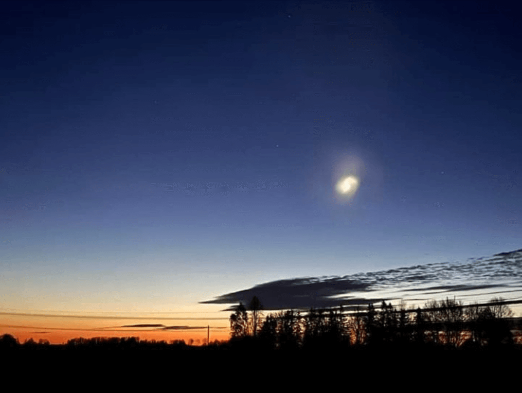
Shortly after the launch, Kairo Kiitsak, a Meteorologist at the Estonian Environment Agency posted the photo below showing what appears to be a sub-orbital rocket component from the launch burning up somewhere over Estonia.
Imagery of Eleven Cities
Maxar have several Basemap products. In this post, I'll be reviewing their Vivid Standard offering. Maxar distributes the eleven cities samples for their Vivid Standard offering as ZIP files. Below are their sizes along with the number of GeoTIFFs they contain, the colour bands used and the resolution buckets of the imagery. They can be downloaded from this link.
| City        | ZIP Size (GB) | # TIFFs | Bands | Res (cm) |
| ----------- | ------------- | ------- | ----- | -------- |
| Sydney      |          11.0 |     118 | RGB   |       50 |
| Lima        |           6.8 |     117 | RGB   |       30 |
| Tokyo       |          11.0 |     108 | RGB   |       50 |
| Auckland    |          22.0 |      92 | BGRN  |       30 |
| Cairo       |           7.1 |      84 | RGB   |       50 |
| Madrid      |           5.2 |      54 | RGB   |       50 |
| San_Diego   |           1.9 |      24 | RGB   |       50 |
| Budapest    |           0.3 |       1 | BGRN  |       50 |
| Kumamoto    |           0.4 |       1 | BGRN  |       50 |
| Los Angeles |           0.4 |       1 | BGRN  |       50 |
| Nairobi     |           0.4 |       1 | BGRN  |       50 |
Each city's ZIP file contains a metadata_strips folder which houses Shapefiles with the metadata for the imagery for each city. I'll load them into a DuckDB table.
$ ~/duckdb maxar.duckdb
CREATE OR REPLACE TABLE maxar AS
                  SELECT 'Auckland'    AS city, * EXCLUDE(geom) FROM ST_READ('Auckland/metadata_strips/Vivid_Standard_30_81ac1591-cc9d-4ada-9f12-91d5f16db23e-APS.shp');

INSERT INTO maxar SELECT 'Budapest'    AS city, * EXCLUDE(geom) FROM ST_READ('Budapest/metadata_strips/Vivid_Standard_2020_sample_Budapest.shp');
INSERT INTO maxar SELECT 'Cairo'       AS city, * EXCLUDE(geom) FROM ST_READ('Cairo/metadata_strips/Vivid_Standard_cdc6a6eb-26d3-4608-a05a-22db86174ff8-APS.shp');
INSERT INTO maxar SELECT 'Kumamoto'    AS city, * EXCLUDE(geom) FROM ST_READ('Kumamoto/metadata_strips/Vivid_Standard_2020_sample_Kumamoto.shp');
INSERT INTO maxar SELECT 'Lima'        AS city, * EXCLUDE(geom) FROM ST_READ('Lima/metadata_strips/Vivid_Standard_30_1768f79f-2894-4deb-acd1-6ec570bce35e-APS.shp');
INSERT INTO maxar SELECT 'Los_Angeles' AS city, * EXCLUDE(geom) FROM ST_READ('Los_Angeles/metadata_strips/Vivid_Standard_2020_sample_Los_Angeles.shp');
INSERT INTO maxar SELECT 'Madrid'      AS city, * EXCLUDE(geom) FROM ST_READ('Madrid/metadata_strips/Vivid_Standard_157be232-35cd-4ee8-b040-f99d3a82a414-APS.shp');
INSERT INTO maxar SELECT 'Nairobi'     AS city, * EXCLUDE(geom) FROM ST_READ('Nairobi/metadata_strips/Vivid_Standard_2020_sample_Nairobi.shp');
INSERT INTO maxar SELECT 'San_Diego'   AS city, * EXCLUDE(geom) FROM ST_READ('San_Diego/metadata_strips/Vivid_Standard_2b0ec064-e90a-441a-ab04-4ede46f78b82-APS.shp');
INSERT INTO maxar SELECT 'Sydney'      AS city, * EXCLUDE(geom) FROM ST_READ('Sydney/metadata_strips/Vivid_Standard_99de141a-ddce-4612-8d27-6ca1027c261b-APS.shp');
INSERT INTO maxar SELECT 'Tokyo'       AS city, * EXCLUDE(geom) FROM ST_READ('Tokyo/metadata_strips/Vivid_Standard_ba59b04c-15fe-4afa-bd3b-62a86117681d-APS.shp');
Below is an example metadata record for a single image taken of Auckland, New Zealand.
$ ~/duckdb maxar.duckdb \
           -json \
           -c "SELECT *
               FROM maxar
               LIMIT 1;" \
    | tail -n1 \
    | jq -S .
[
  {
    "accuracy": 5,
    "acq_date": "2020-08-14",
    "catalog_id": "104001005ED0E900",
    "city": "Auckland",
    "native_res": 0.39,
    "off_nadir": 27.53,
    "proc_notes": null,
    "sensor": "WV03",
    "sun_elev": 34.22
  }
]
Some of the imagery is as old as 2014 but the majority of it was sourced between 2019 and 2021.
CREATE OR REPLACE TABLE acq_years AS
    SELECT   city,
             SUBSTR(acq_date, 0, 5) AS acq_year,
             COUNT(*) num_images
    FROM     maxar
    GROUP BY 1, 2;

WITH pivot_alias AS (
    PIVOT    acq_years
    ON       acq_year
    USING    SUM(num_images)
    GROUP BY city
)
SELECT   *
FROM     pivot_alias
ORDER BY city;
┌─────────────┬────────┬────────┬────────┬────────┬────────┬────────┬────────┬────────┐
│    city     │  2014  │  2016  │  2017  │  2018  │  2019  │  2020  │  2021  │  2022  │
│   varchar   │ int128 │ int128 │ int128 │ int128 │ int128 │ int128 │ int128 │ int128 │
├─────────────┼────────┼────────┼────────┼────────┼────────┼────────┼────────┼────────┤
│ Auckland    │        │        │        │        │        │      6 │     27 │      2 │
│ Budapest    │        │        │        │        │      1 │        │        │        │
│ Cairo       │        │      2 │     15 │     11 │     48 │      9 │        │        │
│ Kumamoto    │        │        │        │        │      4 │      1 │        │        │
│ Lima        │        │        │        │        │        │      2 │      7 │     18 │
│ Los_Angeles │        │        │        │        │        │      3 │        │        │
│ Madrid      │        │        │        │        │      5 │     13 │      5 │        │
│ Nairobi     │        │        │        │        │        │      3 │        │        │
│ San_Diego   │        │        │        │        │      4 │     14 │        │        │
│ Sydney      │      1 │        │      2 │      5 │     15 │     10 │     45 │        │
│ Tokyo       │        │        │        │        │      2 │     36 │     12 │        │
├─────────────┴────────┴────────┴────────┴────────┴────────┴────────┴────────┴────────┤
│ 11 rows                                                                   9 columns │
└─────────────────────────────────────────────────────────────────────────────────────┘
Their WorldView-4 (WV04) satellite only produced a single image for Cairo, Egypt while WorldView-2 (WV02) was responsible for the lion's share of imagery.
WITH pivot_alias AS (
    PIVOT    maxar
    ON       sensor
    USING    COUNT(*)
    GROUP BY city
)
SELECT   *
FROM     pivot_alias
ORDER BY city;
┌─────────────┬───────┬───────┬───────┬───────┐
│    city     │ GE01  │ WV02  │ WV03  │ WV04  │
│   varchar   │ int64 │ int64 │ int64 │ int64 │
├─────────────┼───────┼───────┼───────┼───────┤
│ Auckland    │    11 │    13 │    11 │     0 │
│ Budapest    │     0 │     1 │     0 │     0 │
│ Cairo       │    16 │    46 │    22 │     1 │
│ Kumamoto    │     0 │     5 │     0 │     0 │
│ Lima        │     9 │    12 │     6 │     0 │
│ Los_Angeles │     1 │     2 │     0 │     0 │
│ Madrid      │     1 │    15 │     7 │     0 │
│ Nairobi     │     1 │     2 │     0 │     0 │
│ San_Diego   │     8 │     5 │     5 │     0 │
│ Sydney      │    17 │    45 │    16 │     0 │
│ Tokyo       │     4 │    36 │    10 │     0 │
├─────────────┴───────┴───────┴───────┴───────┤
│ 11 rows                           5 columns │
└─────────────────────────────────────────────┘
BGRN: Blue + Green + Red + Near-IR
Six of the cities are in RGB format and will load correctly in QGIS without issue. But five cities are in BGRN (Blue + Green + Red + Near-IR). When you load them into QGIS they'll look as though they've been tinted blue. Below is a comparison between Google Earth and Maxar's Basemap for Los Angeles.
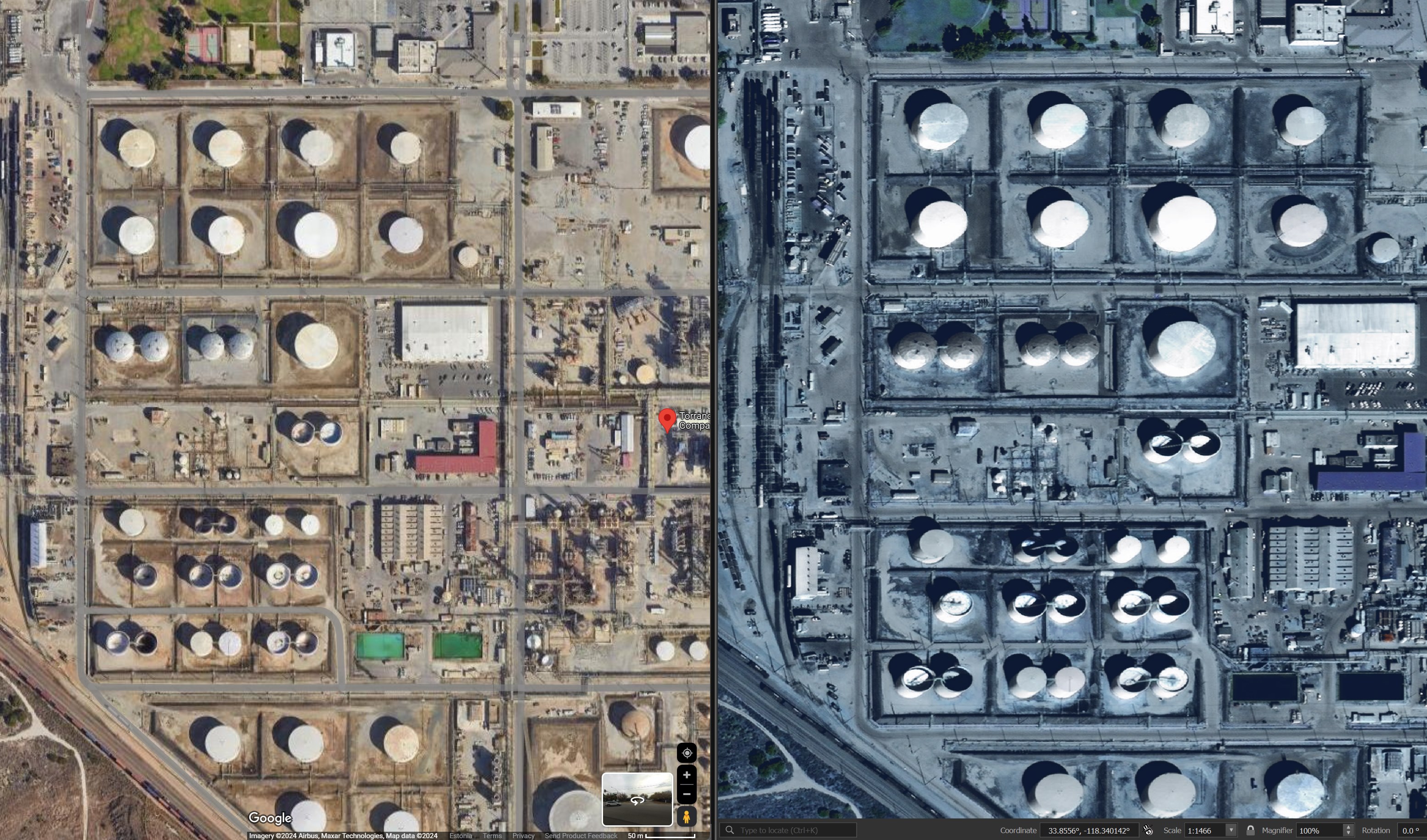
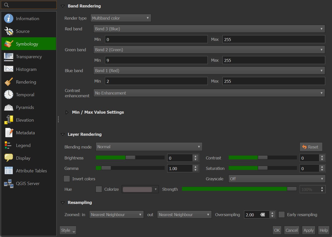
To correct the colour, open the symbology pane for the image and swap the assignments for the red and blue channels.
Cloud-Optimised GeoTIFFs
The TIFF files Maxar delivers are Cloud-Optimised GeoTIFF containers. The files contain Tiled Multi-Resolution TIFFs / Tiled Pyramid TIFFs. This means there are several versions of the same image at different resolutions within the TIFF file.
These files are structured so it's easy to only read a portion of a file for any one resolution you're interested in. A file might be 100 MB but a JavaScript-based Web Application might only need to download 2 MB of data from that file in order to render its lowest resolution.
Below I'll write a parser to convert the output from tiffinfo into JSON.
$ vi tiff_json.py
from   glob          import glob
import json
from   pathlib       import Path
import re
from   shlex         import quote

from   rich.progress import track
from   shpyx         import run as execute


def parse_tiff(lines:list):
    stack, stack_id = {}, None

    for line in lines:
        if not stack_id:
            stack_id = 1
        elif line.startswith('TIFF Directory'):
            stack_id = stack_id + 1
        elif line.startswith('  ') and line.count(':') == 1:
            if stack_id not in stack:
                stack[stack_id] = {'stack_num': stack_id}

            x, y = line.strip().split(':')

            if len(x) > 1 and not x.startswith('Tag ') and \
               y and \
               len(str(y).strip()) > 1:
                stack[stack_id][x.strip()] = y.strip()
        elif line.startswith('  ') and \
             line.count(':') == 2 and \
             'Image Width' in line:
            if stack_id not in stack:
                stack[stack_id] = {'stack_num': stack_id}

            _, width, _, _, _ = re.split(r'\: ([0-9]*)', line)
            stack[stack_id]['width'] = int(width.strip())

    return [y for x, y in stack.items()]


with open('maxar_imagery.jsonl', 'w') as f:
    for path in track(glob('*/raster_tiles/*.tif')):
        lines = execute('tiffinfo -i %s' % quote(path))\
                    .stdout\
                    .strip()\
                    .splitlines()

        for line in parse_tiff(lines):
            f.write(json.dumps({**line,
                                **{'filename': path}},
                               sort_keys=True) + '\n')
$ python tiff_json.py
I'll load the metadata extracted above into DuckDB.
$ ~/duckdb maxar.duckdb
CREATE OR REPLACE TABLE geotiffs AS
    SELECT *
    FROM   READ_JSON('maxar_imagery.jsonl');
I'll create separate tables for the transparency and colour stacks.
CREATE OR REPLACE TABLE geotiffs_masks AS
    SELECT *
    FROM   geotiffs
    WHERE  "Photometric Interpretation" = 'transparency mask';

CREATE OR REPLACE TABLE geotiffs_colour AS
    SELECT *
    FROM   geotiffs
    WHERE  "Photometric Interpretation" != 'transparency mask';
Below you can see the various widths supported across each of the stacks for the transparency masks.
WITH pivot_alias AS (
    PIVOT    geotiffs_masks
    ON       FORMAT('{:02d}', stack_num)
    USING    COUNT(*)
    GROUP BY width
)
SELECT   *
FROM     pivot_alias
ORDER BY width;
┌───────┬───────┬───────┬───────┬───────┬───────┬───────┬───────┐
│ width │  02   │  09   │  10   │  11   │  12   │  13   │  14   │
│ int64 │ int64 │ int64 │ int64 │ int64 │ int64 │ int64 │ int64 │
├───────┼───────┼───────┼───────┼───────┼───────┼───────┼───────┤
│   256 │     0 │     0 │     0 │     0 │     0 │     0 │   209 │
│   306 │     0 │     0 │     0 │     0 │     0 │     0 │   392 │
│   512 │     0 │     0 │     0 │     0 │     0 │   209 │     0 │
│   612 │     0 │     0 │     0 │     0 │     0 │   392 │     0 │
│  1024 │     0 │     0 │     0 │     0 │   209 │     0 │     0 │
│  1224 │     0 │     0 │     0 │     0 │   392 │     0 │     0 │
│  2048 │     0 │     0 │     0 │   209 │     0 │     0 │     0 │
│  2448 │     0 │     0 │     0 │   392 │     0 │     0 │     0 │
│  4096 │     0 │     0 │   209 │     0 │     0 │     0 │     0 │
│  4896 │     0 │     0 │   392 │     0 │     0 │     0 │     0 │
│  8192 │     0 │   209 │     0 │     0 │     0 │     0 │     0 │
│  9792 │     0 │   392 │     0 │     0 │     0 │     0 │     0 │
│ 16384 │   209 │     0 │     0 │     0 │     0 │     0 │     0 │
│ 19584 │   392 │     0 │     0 │     0 │     0 │     0 │     0 │
├───────┴───────┴───────┴───────┴───────┴───────┴───────┴───────┤
│ 14 rows                                             8 columns │
└───────────────────────────────────────────────────────────────┘
These are the widths supported for the RGB & YCbCr stacks.
WITH pivot_alias AS (
    PIVOT    geotiffs_colour
    ON       FORMAT('{:02d}', stack_num)
    USING    COUNT(*)
    GROUP BY width
)
SELECT   *
FROM     pivot_alias
ORDER BY width;
┌───────┬───────┬───────┬───────┬───────┬───────┬───────┬───────┐
│ width │  01   │  03   │  04   │  05   │  06   │  07   │  08   │
│ int64 │ int64 │ int64 │ int64 │ int64 │ int64 │ int64 │ int64 │
├───────┼───────┼───────┼───────┼───────┼───────┼───────┼───────┤
│   256 │     0 │     0 │     0 │     0 │     0 │     0 │   209 │
│   306 │     0 │     0 │     0 │     0 │     0 │     0 │   392 │
│   512 │     0 │     0 │     0 │     0 │     0 │   209 │     0 │
│   612 │     0 │     0 │     0 │     0 │     0 │   392 │     0 │
│  1024 │     0 │     0 │     0 │     0 │   209 │     0 │     0 │
│  1224 │     0 │     0 │     0 │     0 │   392 │     0 │     0 │
│  2048 │     0 │     0 │     0 │   209 │     0 │     0 │     0 │
│  2448 │     0 │     0 │     0 │   392 │     0 │     0 │     0 │
│  4096 │     0 │     0 │   209 │     0 │     0 │     0 │     0 │
│  4896 │     0 │     0 │   392 │     0 │     0 │     0 │     0 │
│  8192 │     0 │   209 │     0 │     0 │     0 │     0 │     0 │
│  9792 │     0 │   392 │     0 │     0 │     0 │     0 │     0 │
│ 16384 │   209 │     0 │     0 │     0 │     0 │     0 │     0 │
│ 19584 │   392 │     0 │     0 │     0 │     0 │     0 │     0 │
├───────┴───────┴───────┴───────┴───────┴───────┴───────┴───────┤
│ 14 rows                                             8 columns │
└───────────────────────────────────────────────────────────────┘
Composite Imagery
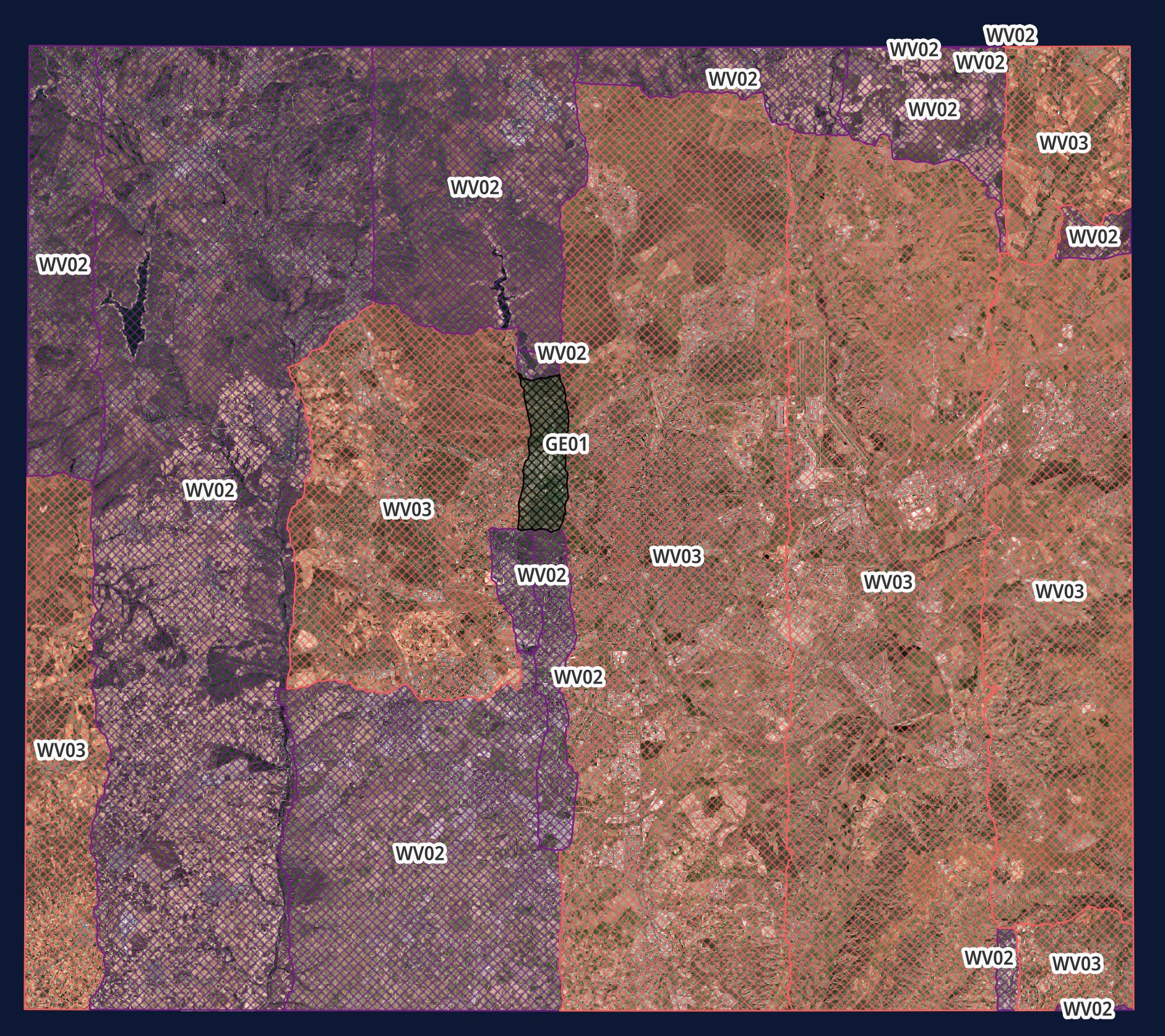
Within any one city, several satellites' imagery will have been composited together to produce the best possible image. Below you can see where GE01, WV02 and WV03 were used for Madrid.
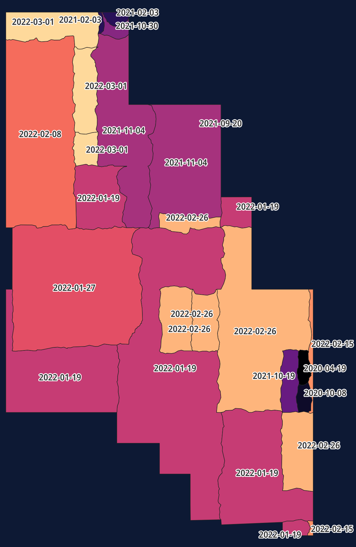
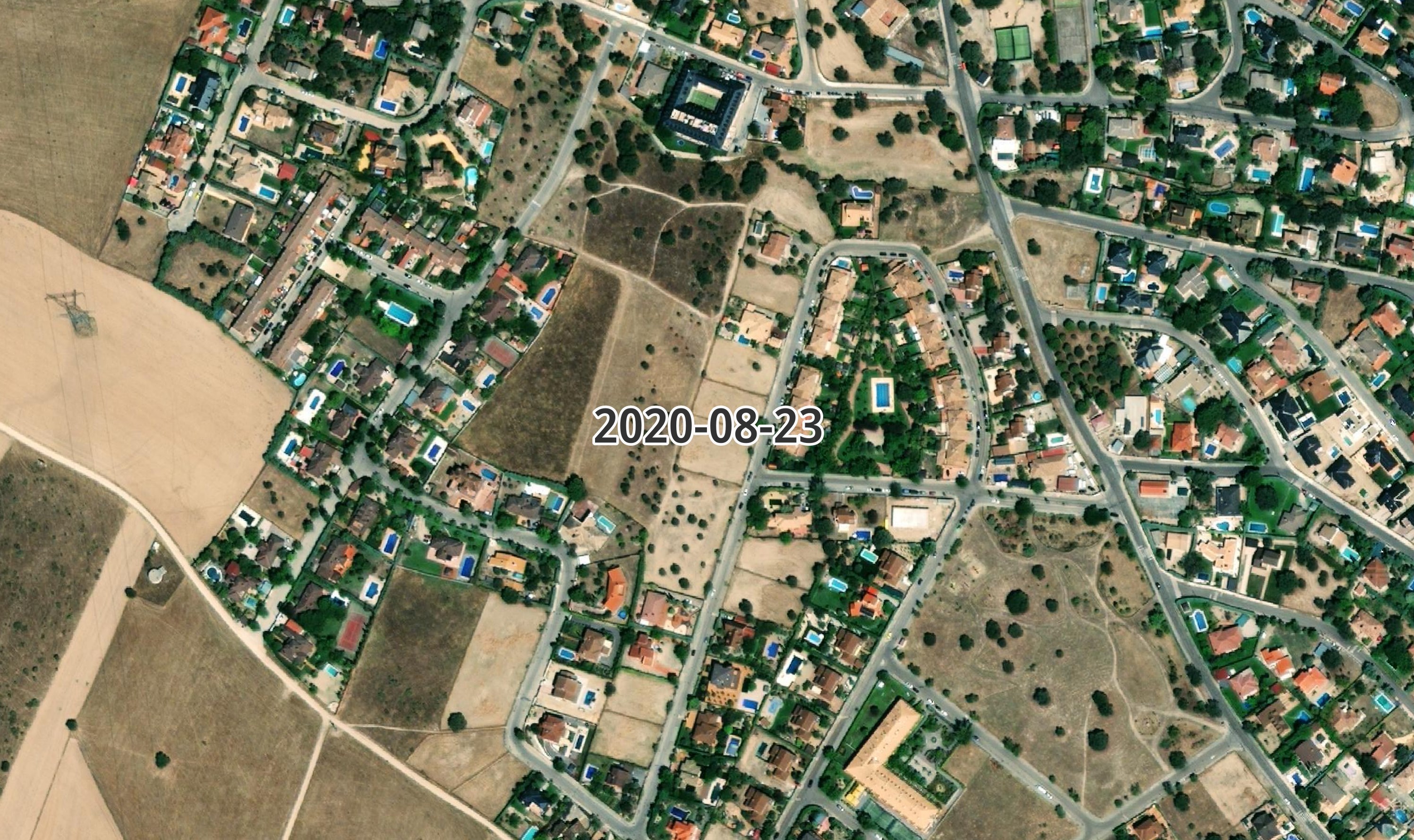
Below are the acquisition dates of the imagery used for Lima.
Below are the native resolutions used for Lima.
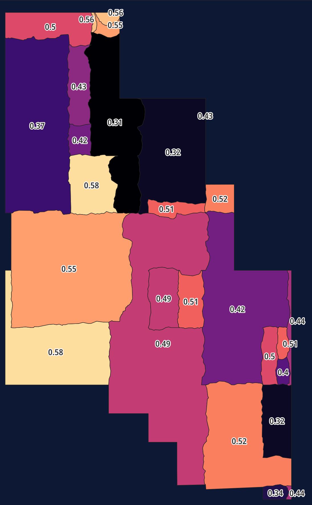
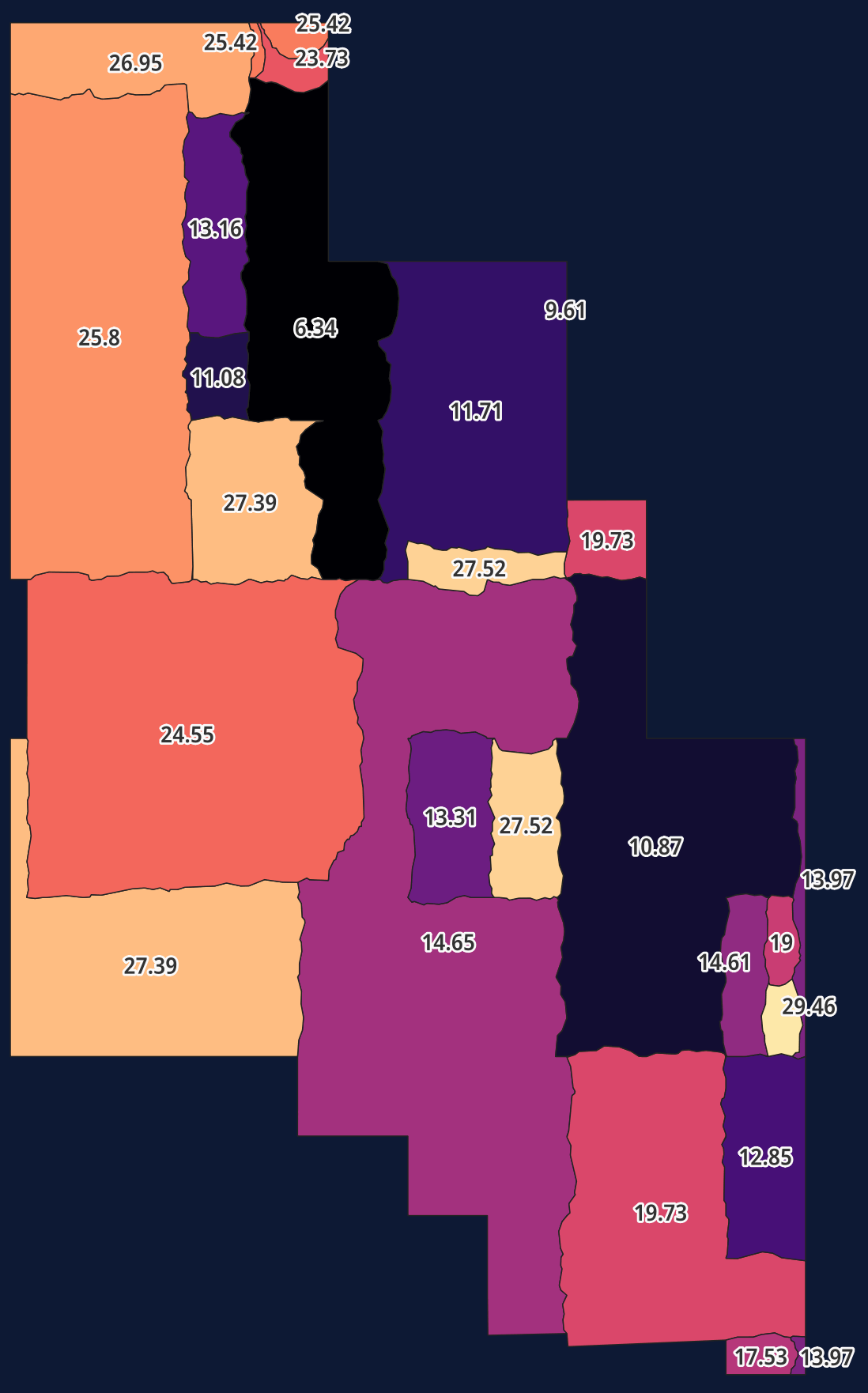
Below are the off-nadir values for Lima.
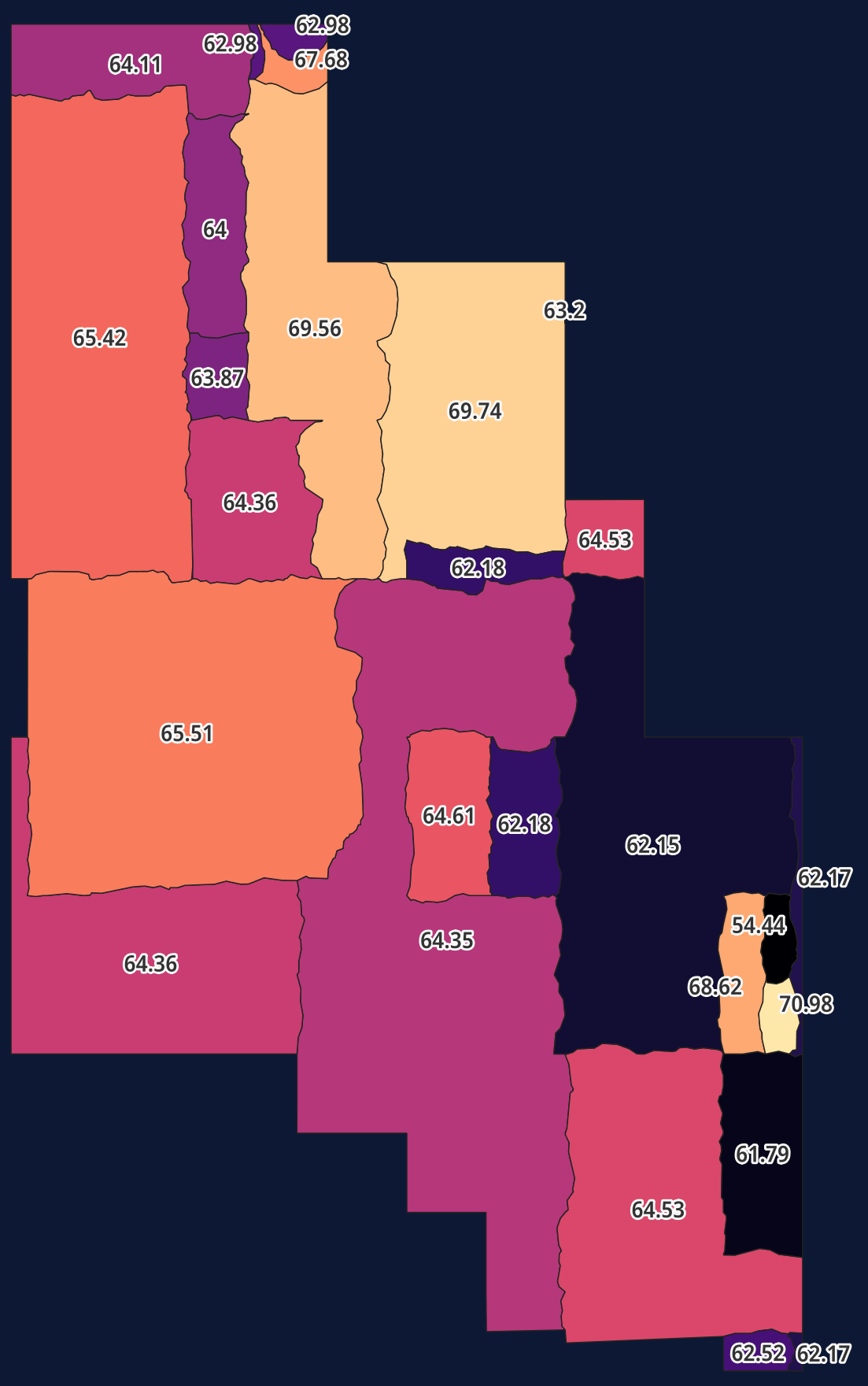
Below are the sun elevation levels for Lima.
Month of Capture
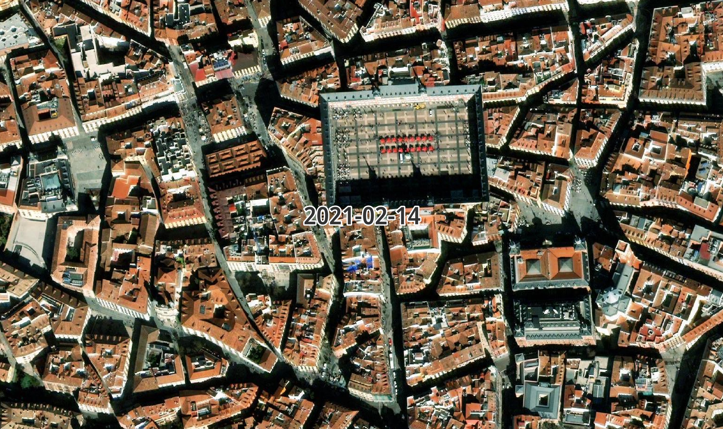
Maxar aimed to use spring and summer imagery as much as possible. Below is an image taken in Madrid in August and shadows are as minimal as can be.
Unfortunately, the imagery for the centre of Madrid was taken in February and the long shadows obscure a lot of streets and squares.
Below are the months in which imagery was used for each city. Sydney has a hotspot around early Autumn as does Cairo.
CREATE OR REPLACE TABLE acq_months AS
    SELECT   city,
             SUBSTR(acq_date, 6, 2) AS month,
             COUNT(*) num_images
    FROM     maxar
    GROUP BY 1, 2;

WITH pivot_alias AS (
    PIVOT    acq_months
    ON       month
    USING    SUM(num_images)
    GROUP BY city
)
SELECT   *
FROM     pivot_alias
ORDER BY city;
┌─────────────┬────────┬────────┬────────┬────────┬────────┬────────┬────────┬────────┬────────┬────────┬────────┬────────┐
│    city     │   01   │   02   │   03   │   04   │   05   │   06   │   07   │   08   │   09   │   10   │   11   │   12   │
│   varchar   │ int128 │ int128 │ int128 │ int128 │ int128 │ int128 │ int128 │ int128 │ int128 │ int128 │ int128 │ int128 │
├─────────────┼────────┼────────┼────────┼────────┼────────┼────────┼────────┼────────┼────────┼────────┼────────┼────────┤
│ Auckland    │      4 │        │      4 │      9 │      4 │        │        │      8 │      1 │      3 │      2 │        │
│ Budapest    │        │        │        │        │        │        │        │        │        │      1 │        │        │
│ Cairo       │     12 │      5 │      2 │      1 │      3 │      5 │     15 │      1 │     12 │     16 │      7 │      6 │
│ Kumamoto    │        │      1 │        │        │      4 │        │        │        │        │        │        │        │
│ Lima        │      7 │     10 │      3 │      1 │        │        │        │        │      1 │      3 │      2 │        │
│ Los_Angeles │        │        │        │        │        │        │        │        │        │        │      3 │        │
│ Madrid      │        │      5 │        │      2 │      4 │      2 │        │      5 │      1 │      4 │        │        │
│ Nairobi     │        │      2 │      1 │        │        │        │        │        │        │        │        │        │
│ San Diego   │      1 │        │      3 │      1 │        │      1 │      3 │        │      1 │      6 │      2 │        │
│ Sydney      │     11 │      5 │      2 │     24 │      7 │      1 │      5 │      1 │     15 │        │      2 │      5 │
│ Tokyo       │      6 │     10 │      1 │     19 │      2 │        │        │      2 │      1 │      2 │      6 │      1 │
├─────────────┴────────┴────────┴────────┴────────┴────────┴────────┴────────┴────────┴────────┴────────┴────────┴────────┤
│ 11 rows                                                                                                      13 columns │
└─────────────────────────────────────────────────────────────────────────────────────────────────────────────────────────┘
To be clear, I don't have access to their entire Basemap dataset so these samples might not be representative of their entire offering.
Resolution isn't everything
The resolutions used for any one city can vary greatly between neighbourhoods. Below are the native resolutions for Madrid.
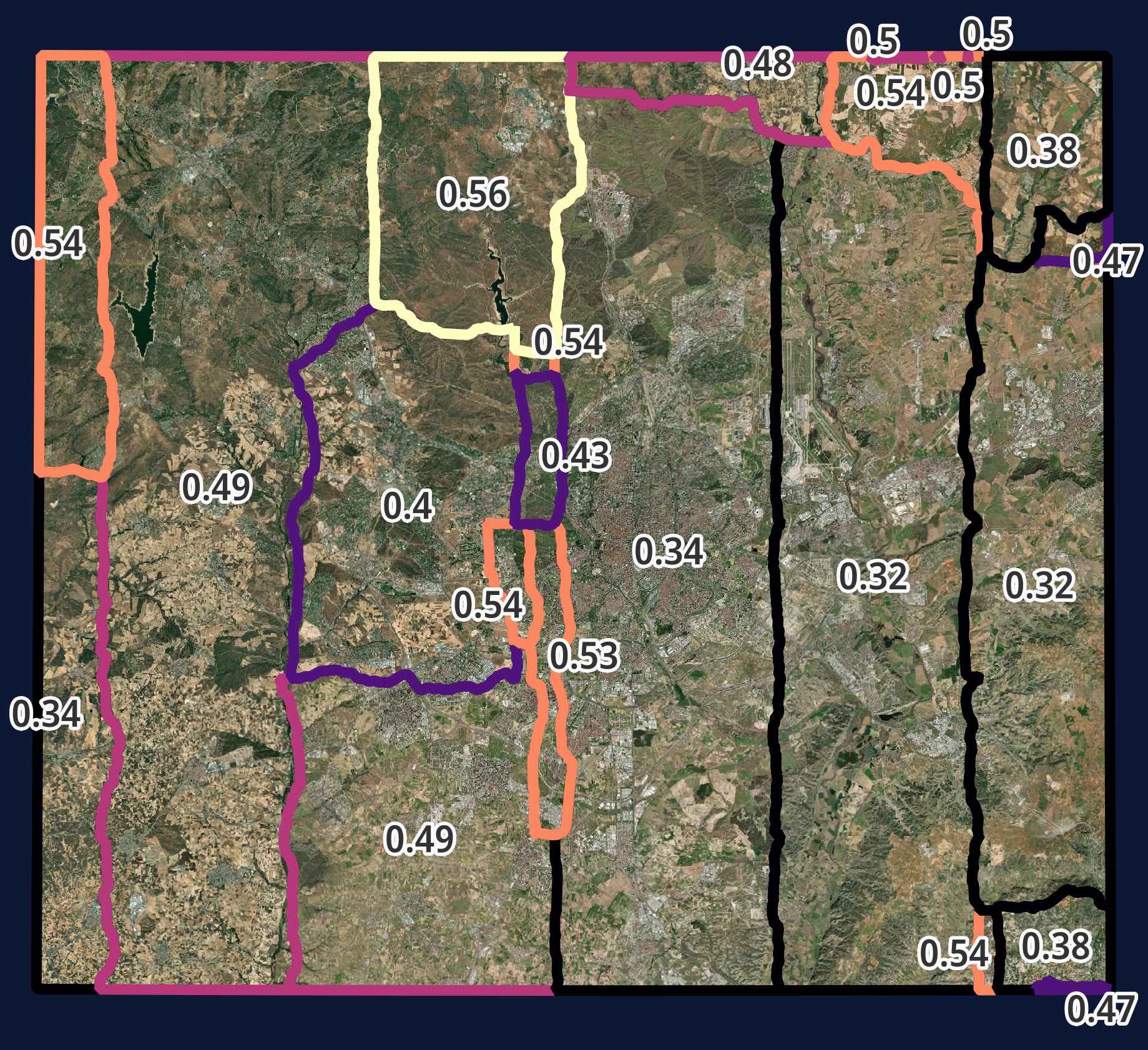
That being said, the resolution isn't the only factor in determining quality. Below the 0.4 and 0.54-meter imagery looks much the same while the 0.43-meter imagery to the top right looks to be of much lower quality.

Below are the native resolution buckets for each city's imagery.
CREATE OR REPLACE TABLE native_res_buckets AS
    SELECT city,
           FORMAT('{:02d}', (ROUND(ROUND(native_res * 100) / 5) * 5)::INT) native_res_bucket,
           COUNT(*) num_images
    FROM maxar
    GROUP BY 1, 2;

WITH pivot_alias AS (
    PIVOT    native_res_buckets
    ON       native_res_bucket
    USING    SUM(num_images)
    GROUP BY city
)
SELECT   *
FROM     pivot_alias
ORDER BY city;
┌─────────────┬────────┬────────┬────────┬────────┬────────┬────────┬────────┐
│    city     │   30   │   35   │   40   │   45   │   50   │   55   │   60   │
│   varchar   │ int128 │ int128 │ int128 │ int128 │ int128 │ int128 │ int128 │
├─────────────┼────────┼────────┼────────┼────────┼────────┼────────┼────────┤
│ Auckland    │        │      8 │      3 │      8 │     10 │      4 │      2 │
│ Budapest    │        │        │        │        │      1 │        │        │
│ Cairo       │      4 │      9 │     13 │      7 │     16 │     26 │     10 │
│ Kumamoto    │        │        │        │        │        │      5 │        │
│ Lima        │      3 │      2 │      3 │      4 │      9 │      4 │      2 │
│ Los_Angeles │        │        │      1 │        │        │      1 │      1 │
│ Madrid      │      2 │      2 │      3 │      3 │      6 │      7 │        │
│ Nairobi     │        │        │      1 │        │      1 │      1 │        │
│ San_Diego   │        │      3 │      4 │      1 │      5 │      3 │      2 │
│ Sydney      │      5 │      9 │      2 │      4 │     21 │     20 │     17 │
│ Tokyo       │      3 │      7 │      1 │      2 │     12 │     19 │      6 │
├─────────────┴────────┴────────┴────────┴────────┴────────┴────────┴────────┤
│ 11 rows                                                          8 columns │
└────────────────────────────────────────────────────────────────────────────┘
Vehicles & Vessels
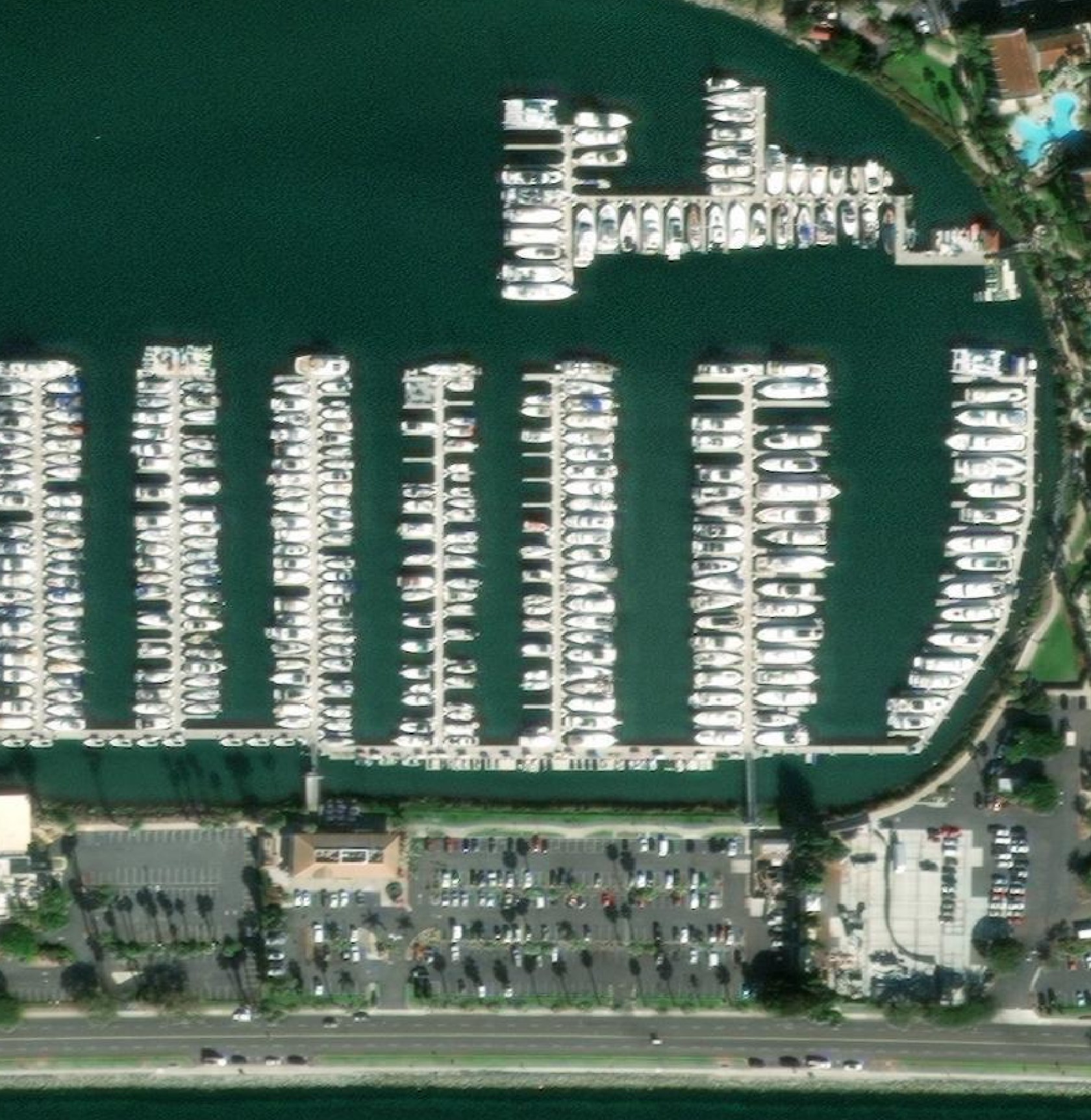
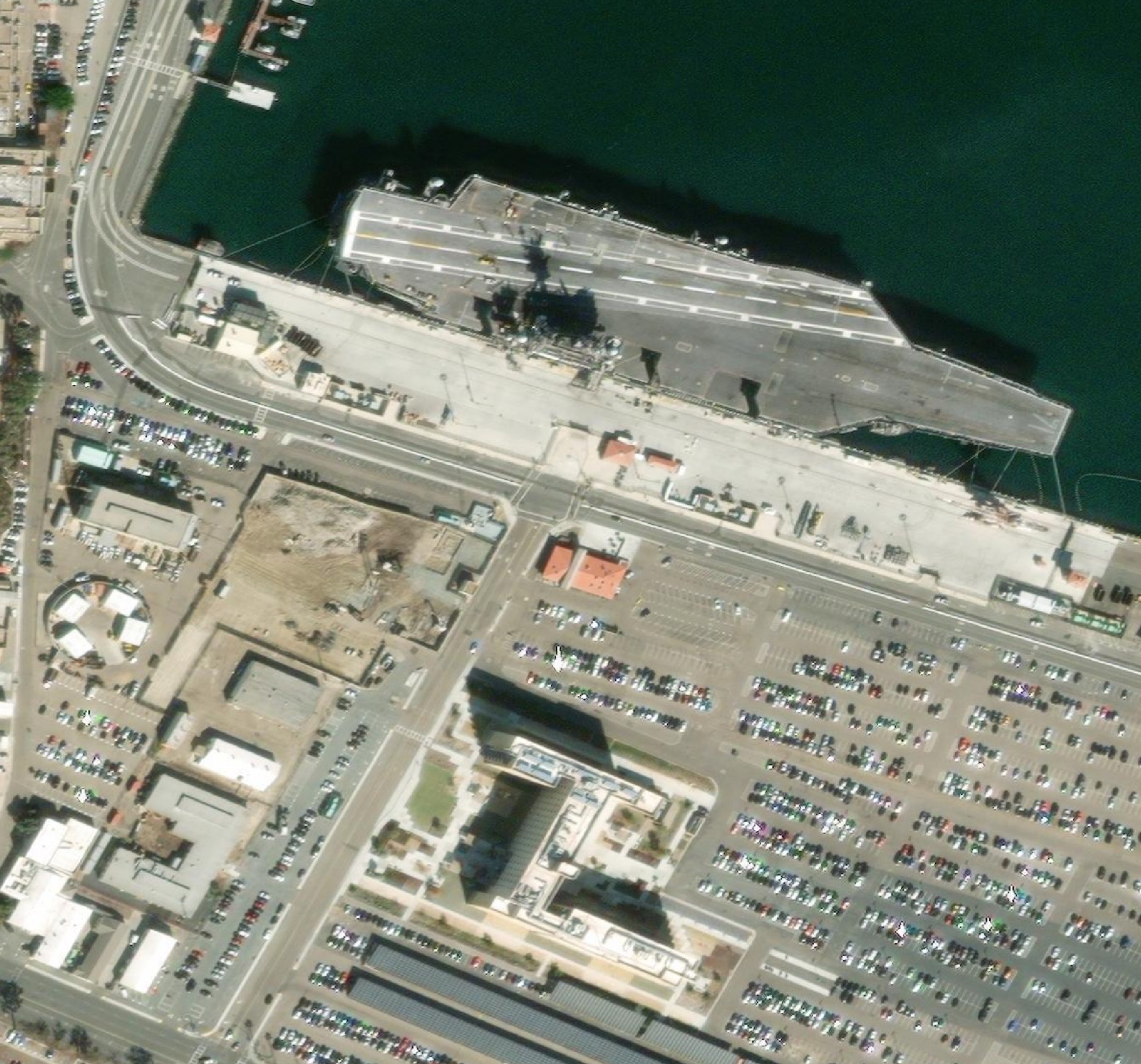
Maxar's imagery of San Diego is good enough to spot individual personal watercraft and cars.
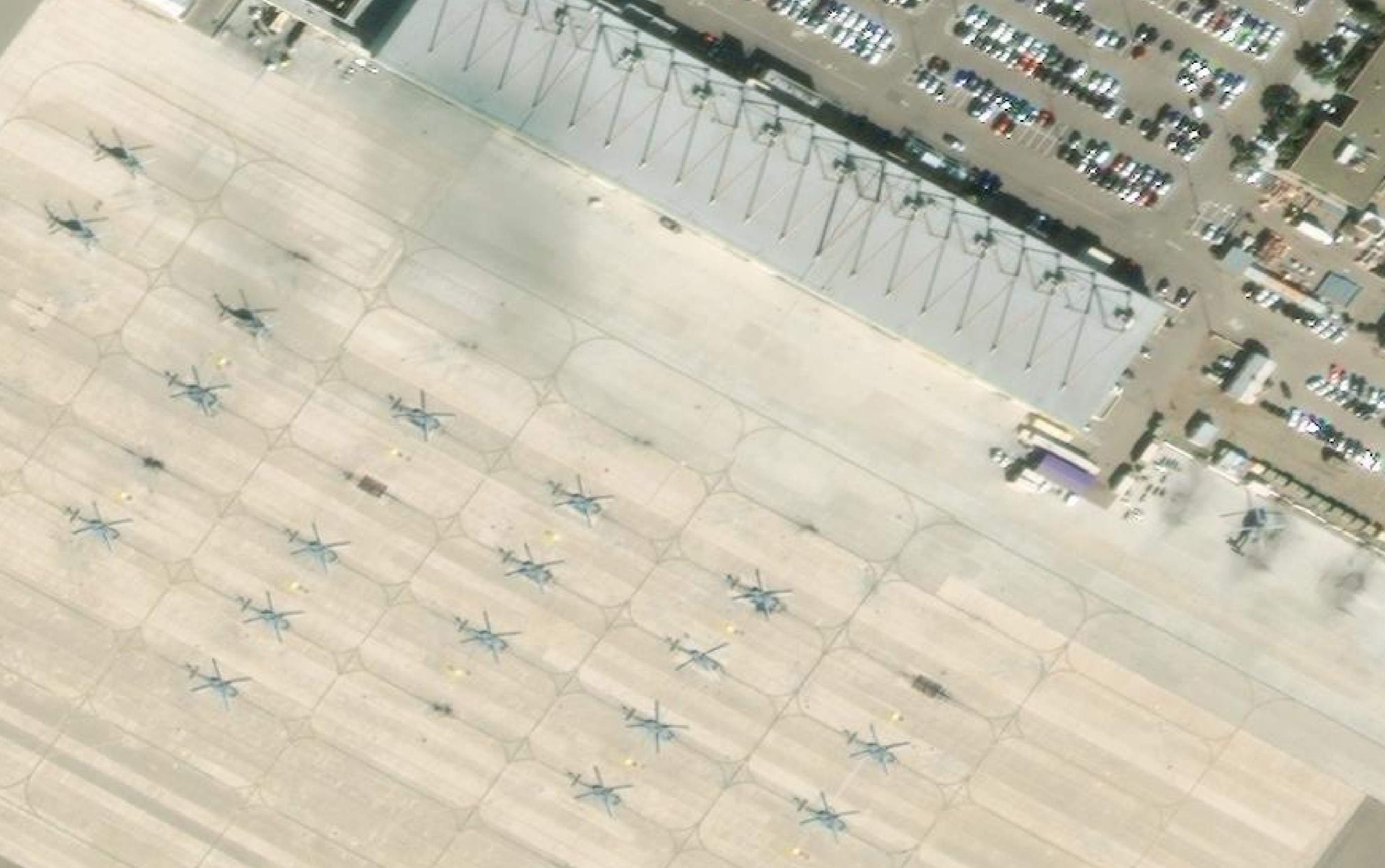
Helicopters appear reasonably clear and might not be too difficult for AI to identify.
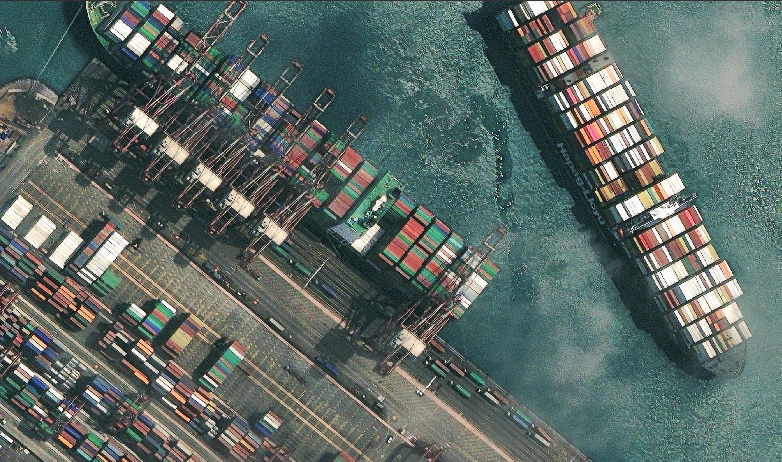
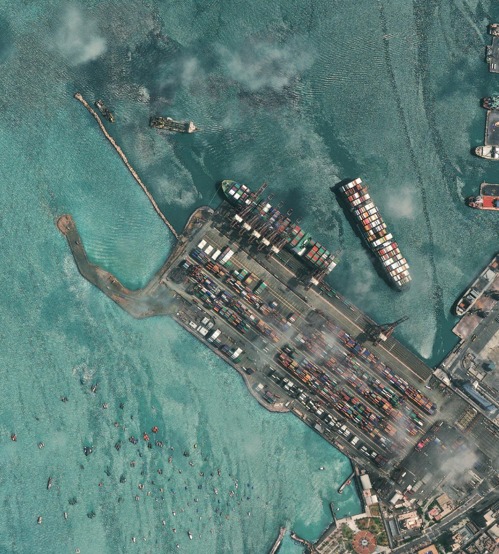
Shipping containers in Lima are clearly visible and it might be possible for AI to count how many are on any given ship and/or stacked up in the port.
Aircraft carriers stick out like a sore thumb.
Oceans & Seas
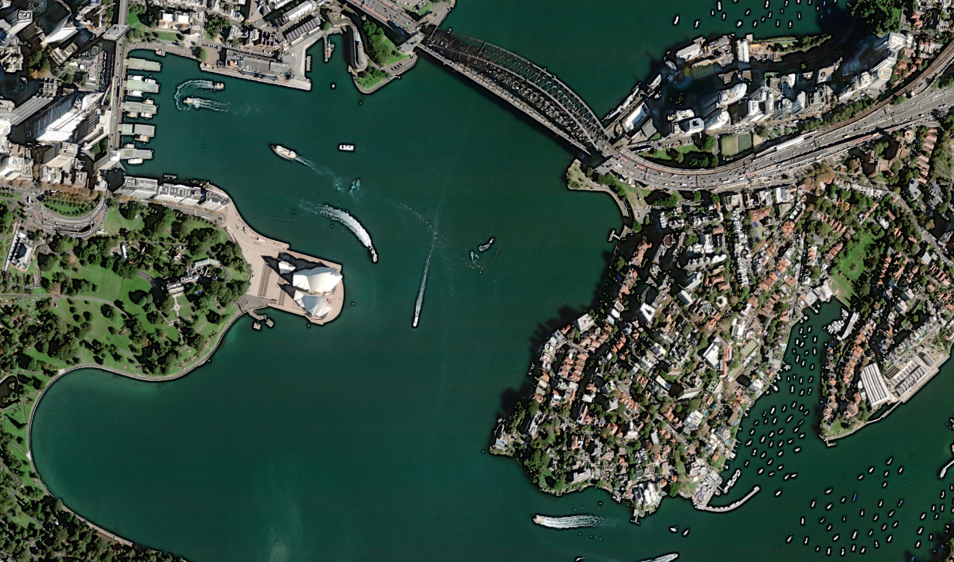
Google Maps' obscures open oceans and seas very close to the coastline. It's nice to see Maxar leave a lot more margin so more of the sea, and the boats sailing on them are visible further away from shore than they would be with Google.
The amount of ocean visible off of San Diego is pretty substantial.
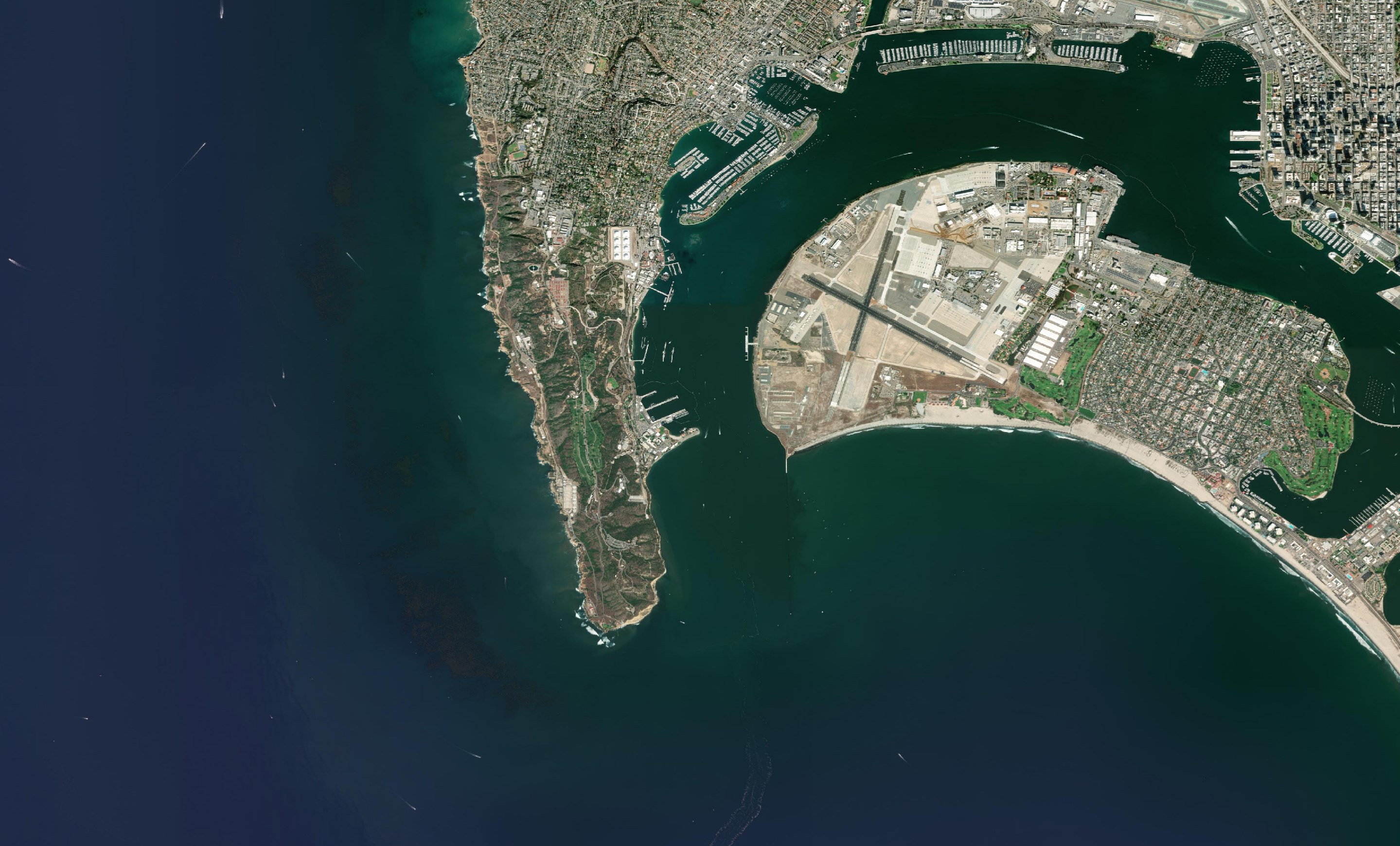
When Maxar does start to obscure the open ocean, they pick a very tasteful shade of blue to do so.
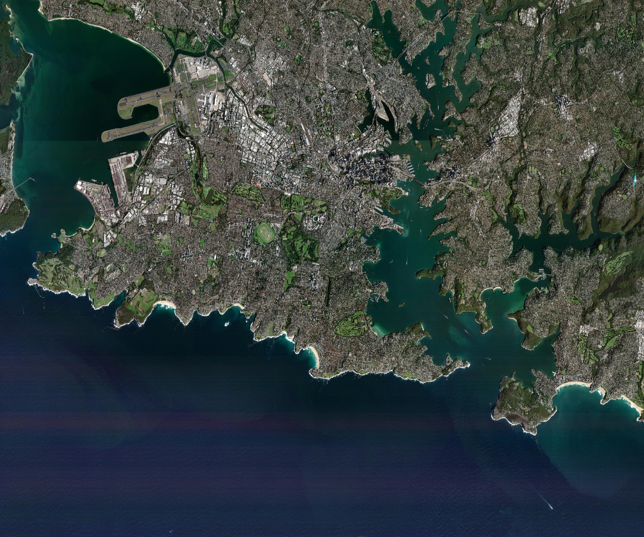
While looking into this, I noticed a lot of watercraft and shorelines in Sydney's Harbour appear to have a black outline around them. I'm not completely sure as to why this is.
Buildings Obstructing Streets
"Off-Nadir" is the satellite's angle in relation to the ground. The larger the angle, the more pixels get stretched so there is a relationship between this value and how useable the resulting image is.
I noticed for Sydney's Central Business District that the tall buildings were caught at such an angle that it's very difficult to see the streets below them.
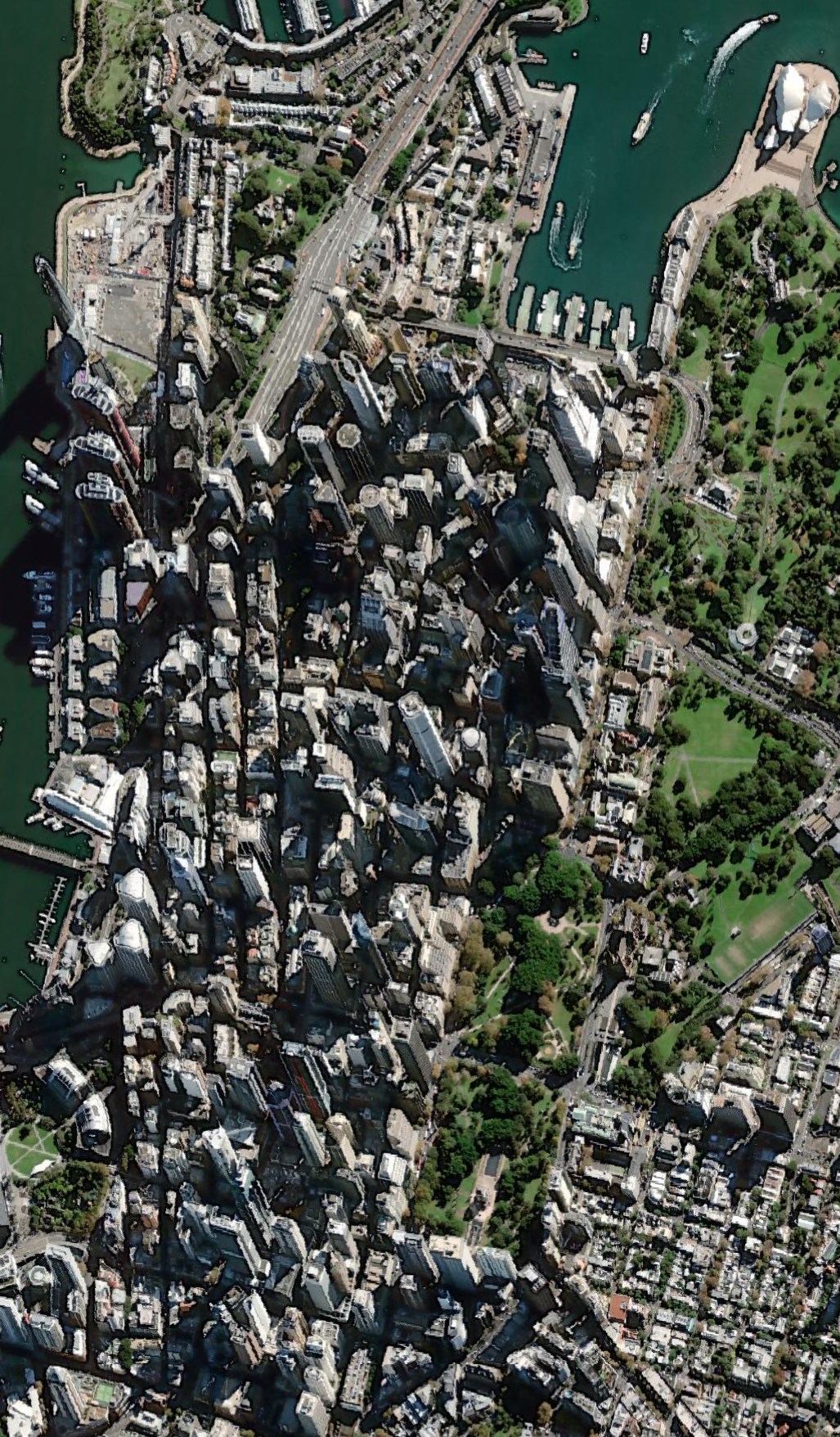
Much of the Sydney imagery was captured around 25-30 degrees.
CREATE OR REPLACE TABLE off_nadir_buckets AS
    SELECT   city,
             FORMAT('{:02d}', (ROUND(ROUND(off_nadir) / 5) * 5)::INT) off_nadir_bucket,
             COUNT(*) num_images
    FROM     maxar
    GROUP BY 1, 2;

WITH pivot_alias AS (
    PIVOT    off_nadir_buckets
    ON       off_nadir_bucket
    USING    SUM(num_images)
    GROUP BY city
)
SELECT   *
FROM     pivot_alias
ORDER BY city;
┌─────────────┬────────┬────────┬────────┬────────┬────────┬────────┬────────┐
│    city     │   00   │   05   │   10   │   15   │   20   │   25   │   30   │
│   varchar   │ int128 │ int128 │ int128 │ int128 │ int128 │ int128 │ int128 │
├─────────────┼────────┼────────┼────────┼────────┼────────┼────────┼────────┤
│ Auckland    │        │        │      6 │      8 │      9 │      7 │      5 │
│ Budapest    │        │        │        │      1 │        │        │        │
│ Cairo       │      1 │      2 │      6 │      5 │     19 │     33 │     19 │
│ Kumamoto    │        │        │        │        │        │      5 │        │
│ Lima        │        │      1 │      4 │      7 │      4 │      8 │      3 │
│ Los_Angeles │        │      1 │        │        │        │      1 │      1 │
│ Madrid      │        │        │      5 │      7 │      2 │      8 │      1 │
│ Nairobi     │        │      1 │        │      1 │      1 │        │        │
│ San_Diego   │        │        │      2 │      1 │      3 │     10 │      2 │
│ Sydney      │      2 │      3 │      2 │      8 │      6 │     43 │     14 │
│ Tokyo       │        │      1 │      2 │      8 │     14 │     20 │      5 │
├─────────────┴────────┴────────┴────────┴────────┴────────┴────────┴────────┤
│ 11 rows                                                          8 columns │
└────────────────────────────────────────────────────────────────────────────┘
Clarity
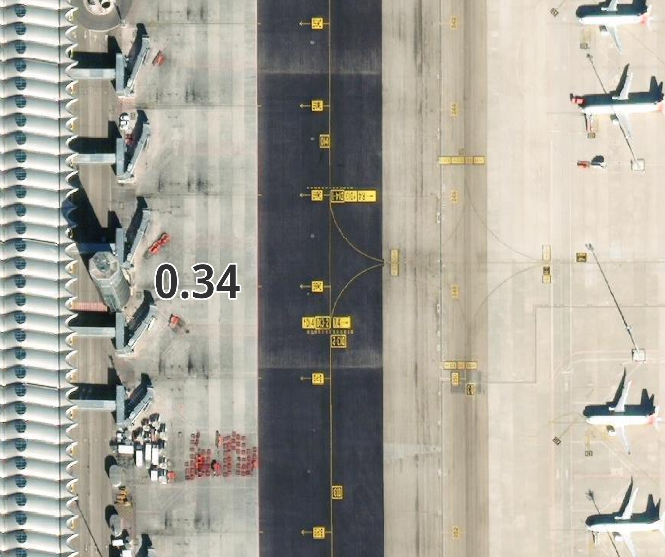
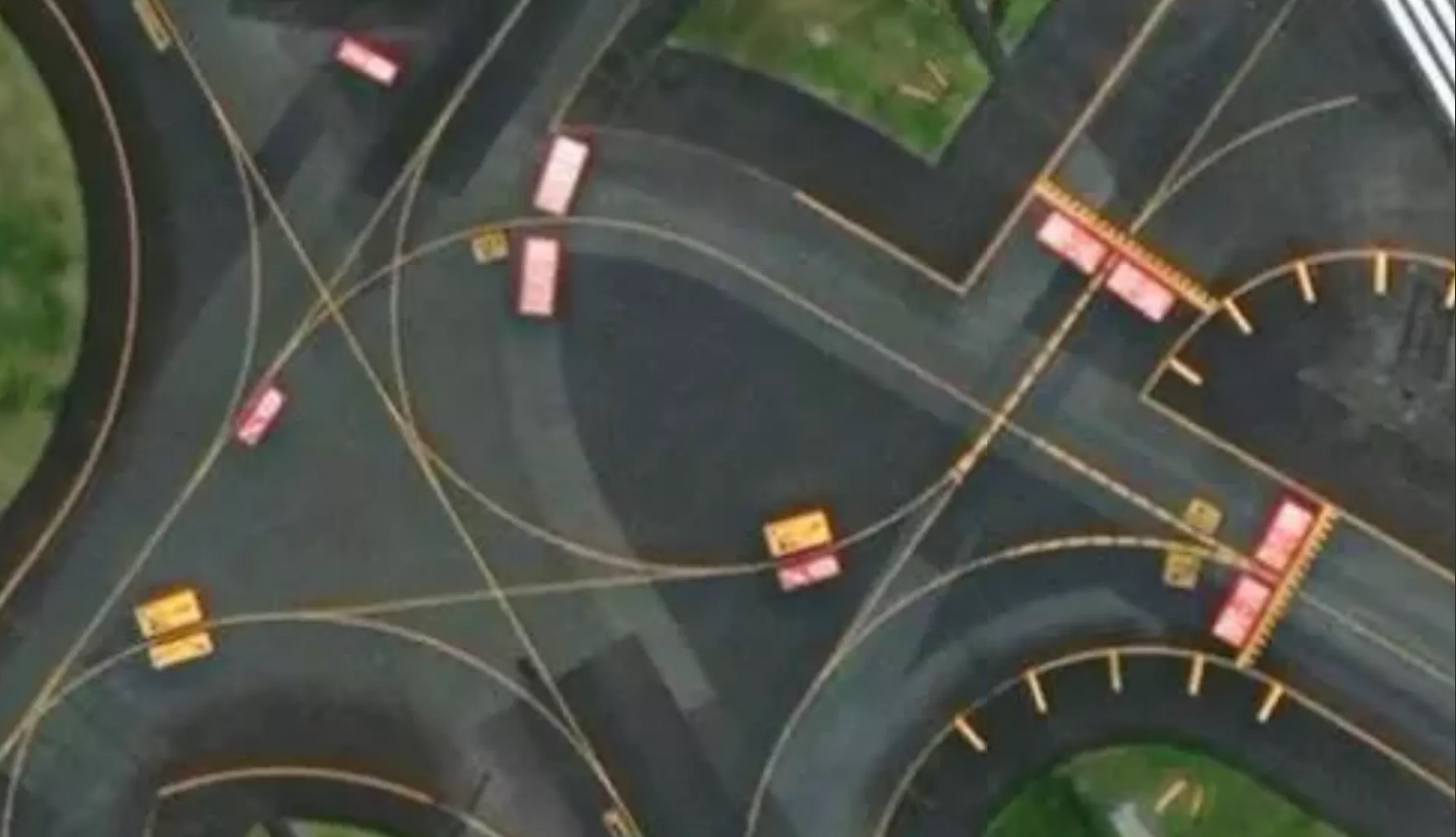
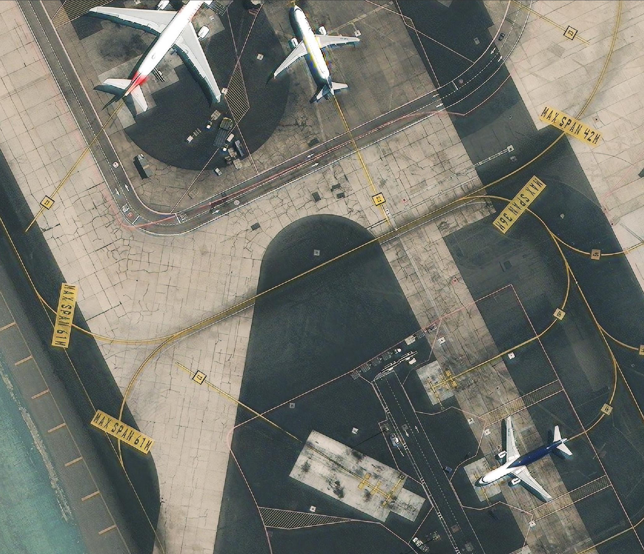
When I examined Madrid's Barajas Airport, the 32-34-cm imagery looked pretty good but I noticed I couldn't read many of the runway markings. This one has a resolution of 34cm.
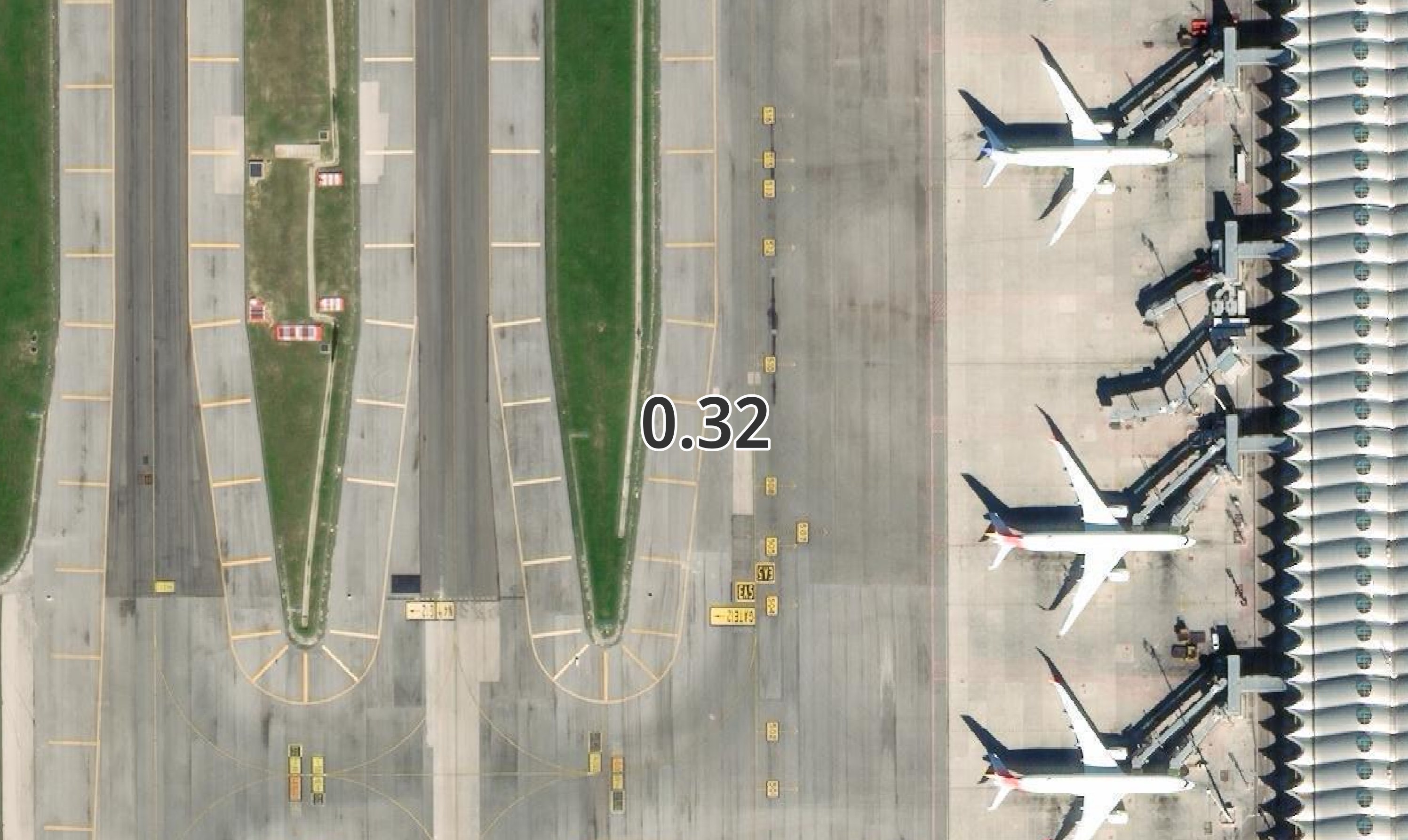
This one is 32cm but not much clearer.
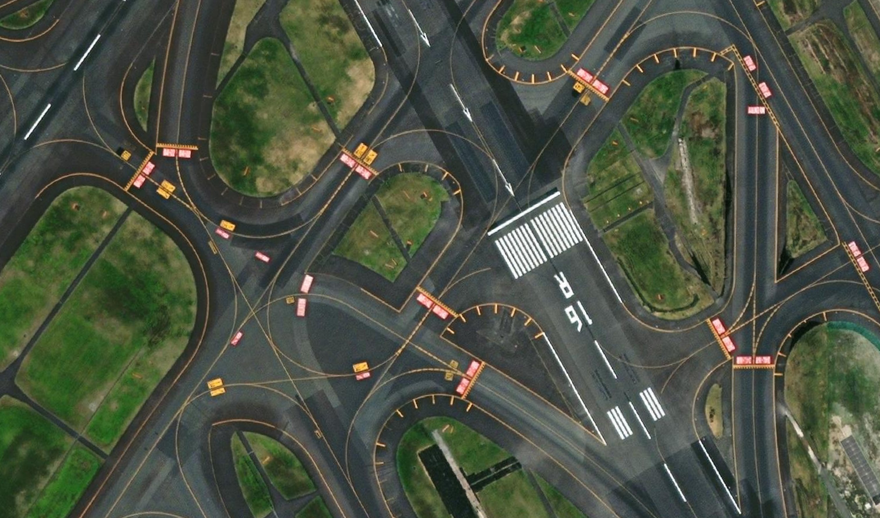
Tokyo's Haneda Airport also looks very clear and seamless when zoomed out.
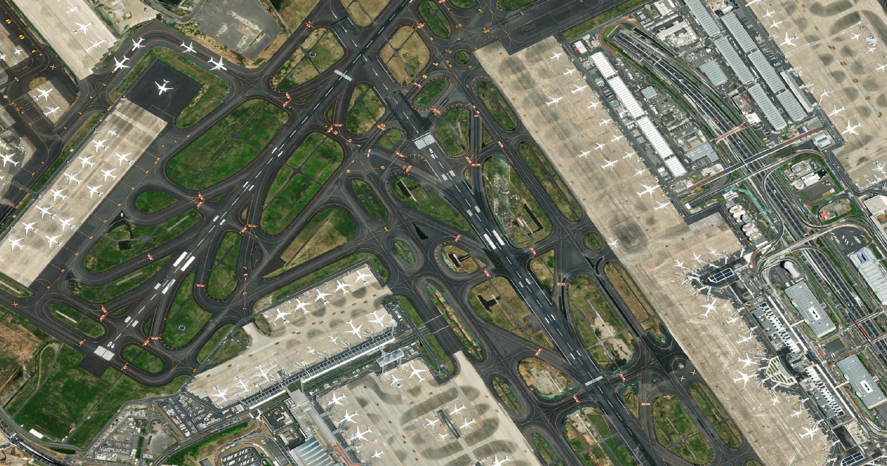
However many of the runway markings are also not completely clear.
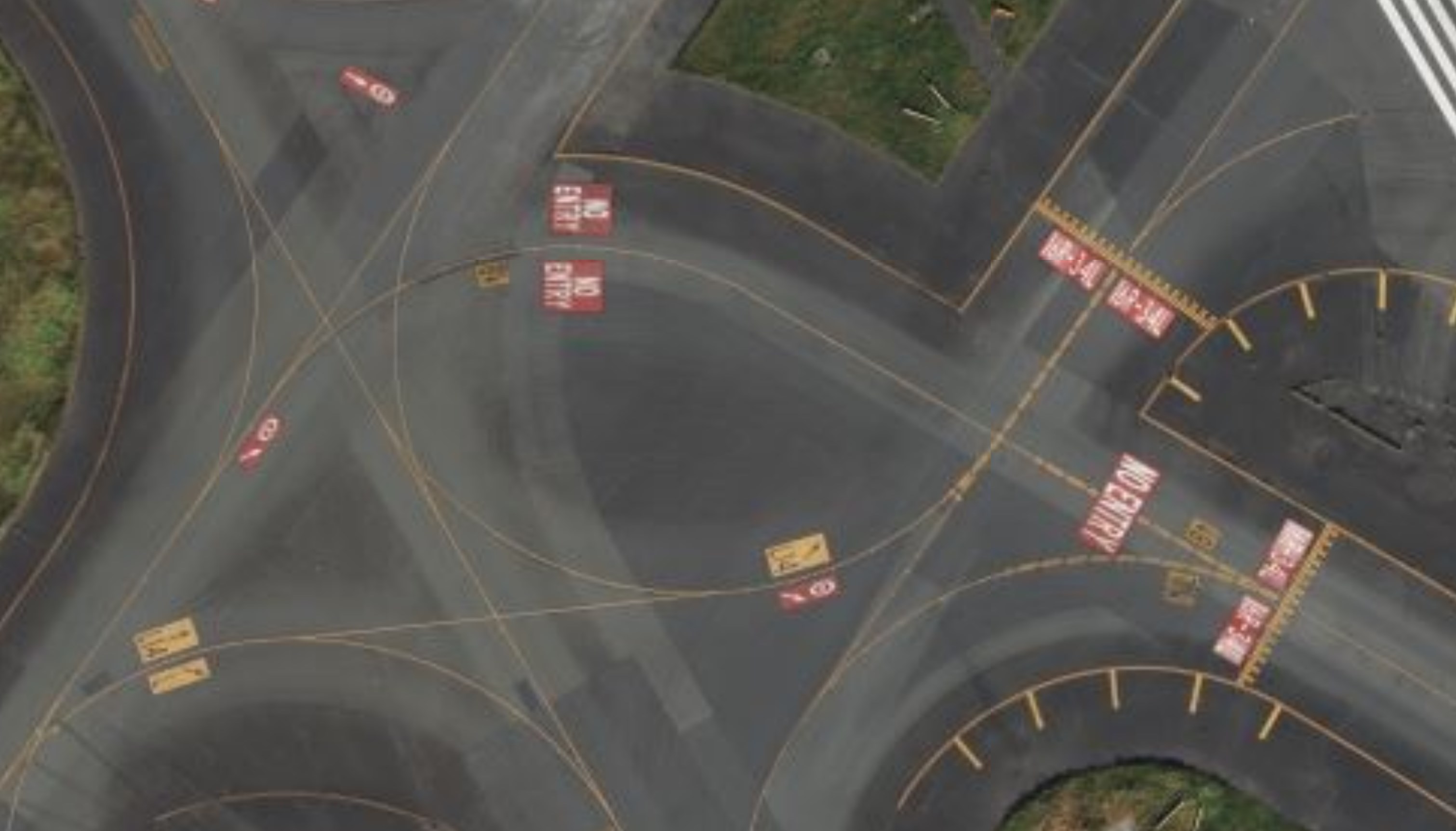
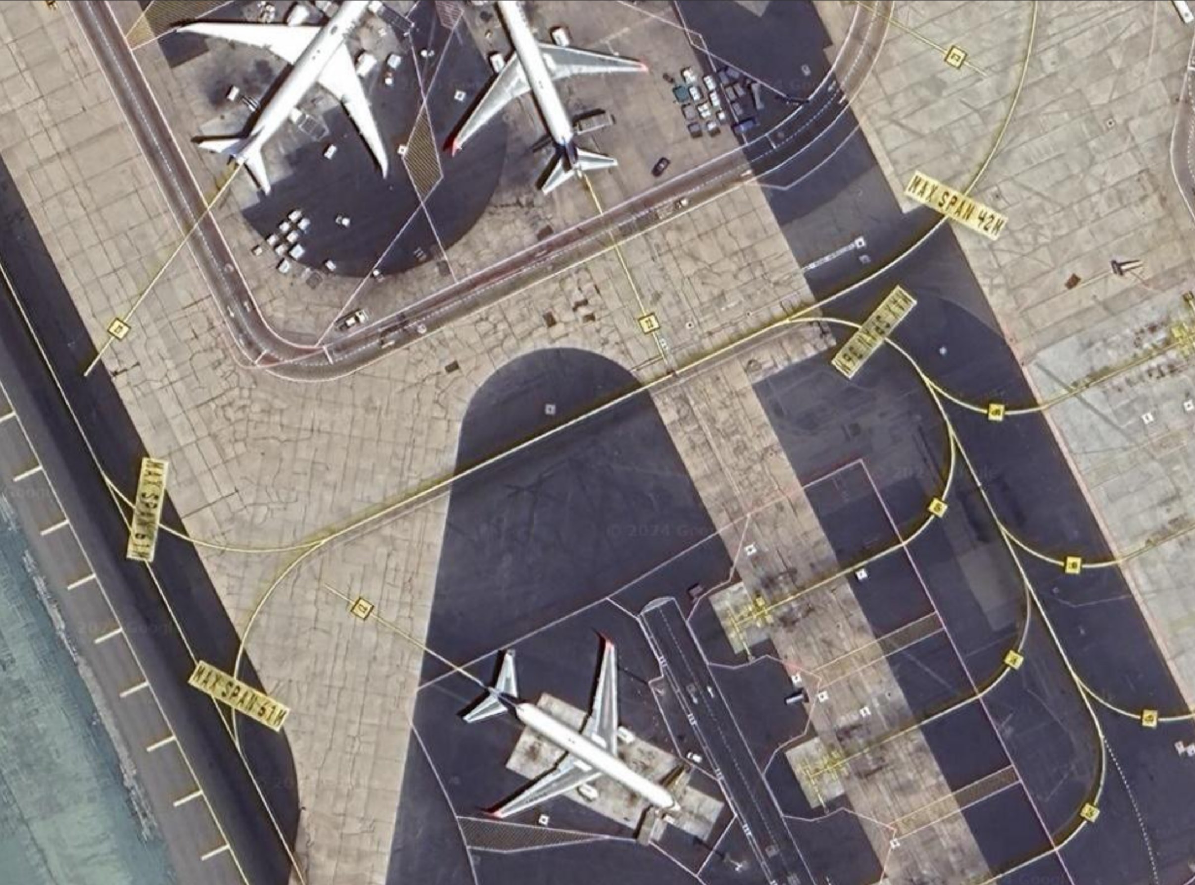
I looked at the same runway location on Google Maps and every marking on the runway is very clear. The credit for the image was given to both Airbus and Maxar but these companies compete against one another and it's likely Google produced a composite from their respective imagery.
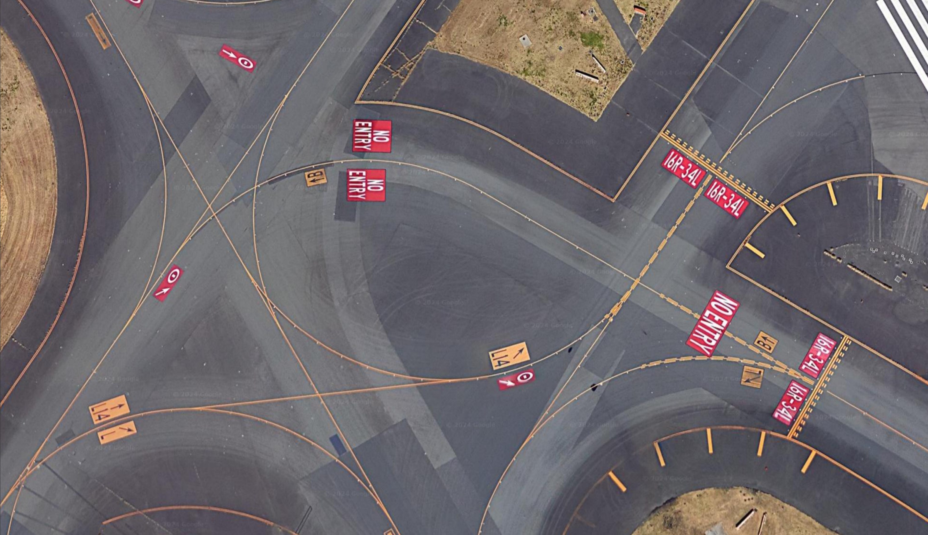
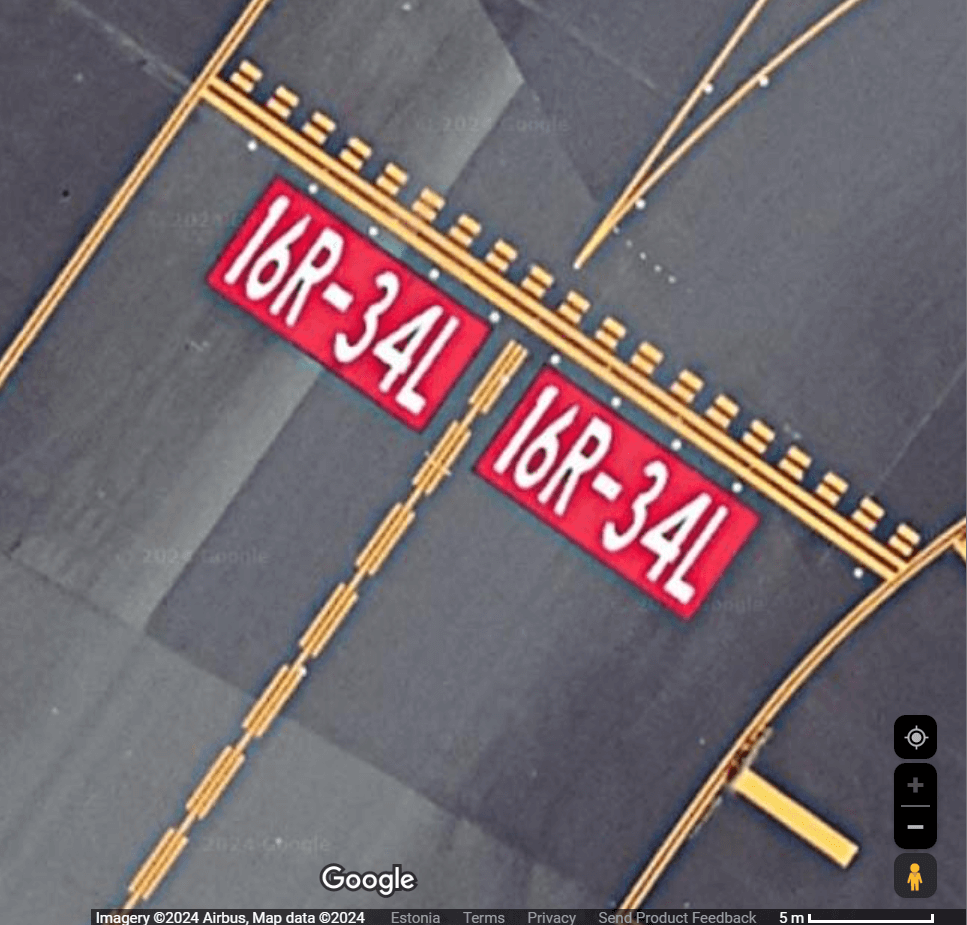
When I zoomed into one of the markings as close as I could in Google Maps, I could see the attribution went to Airbus, not Maxar. Each red marking is ~6-7-meters wide so it should be visible even with 50cm-resolution imagery. I'm not sure what other enhancements Google and/or Airbus might have made to get the markings to come out so clearly.
For comparison, this is MapBox's imagery for the same location.
Bing Maps' is almost legible.
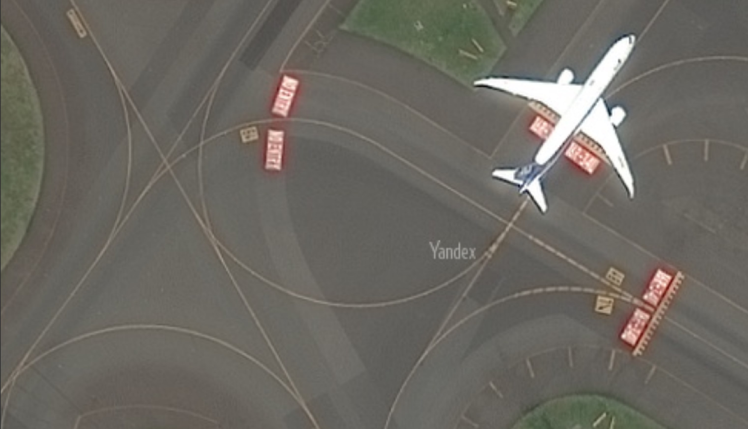
Yandex's is almost legible as well.
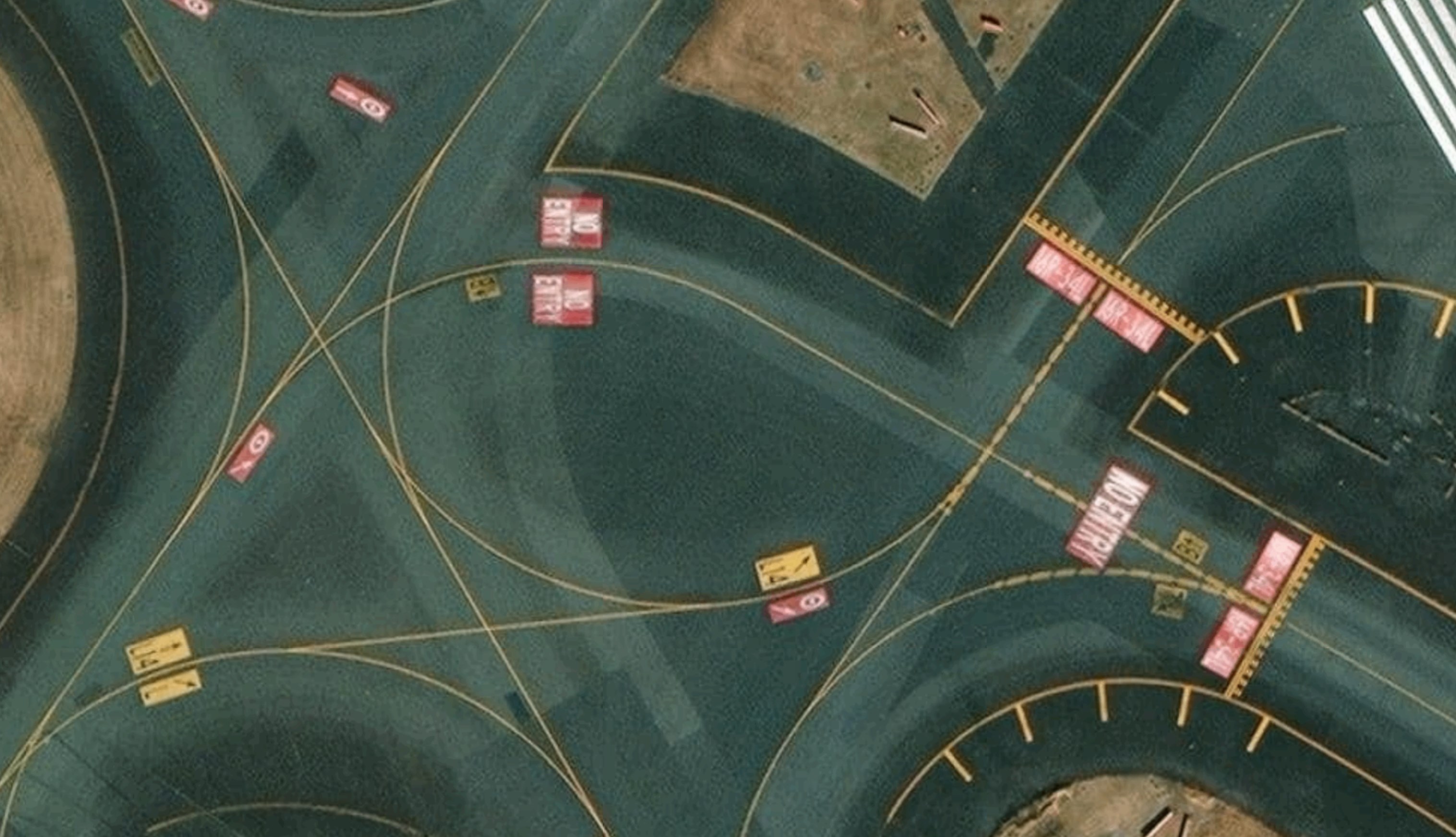
HERE's imagery is probably the most legible after Google's
Standard versus Premium
After I initially published this post, I looked at the samples from Maxar's Premium Basemap offering. The sample cities doesn't include Tokyo but it does include Lima. Below is Lima's Airport in the standard offering.

And below is the premium offering. The runway markings are much more legible and I'd consider this slightly ahead of Google Maps.
Below is Google's imagery from the same location.
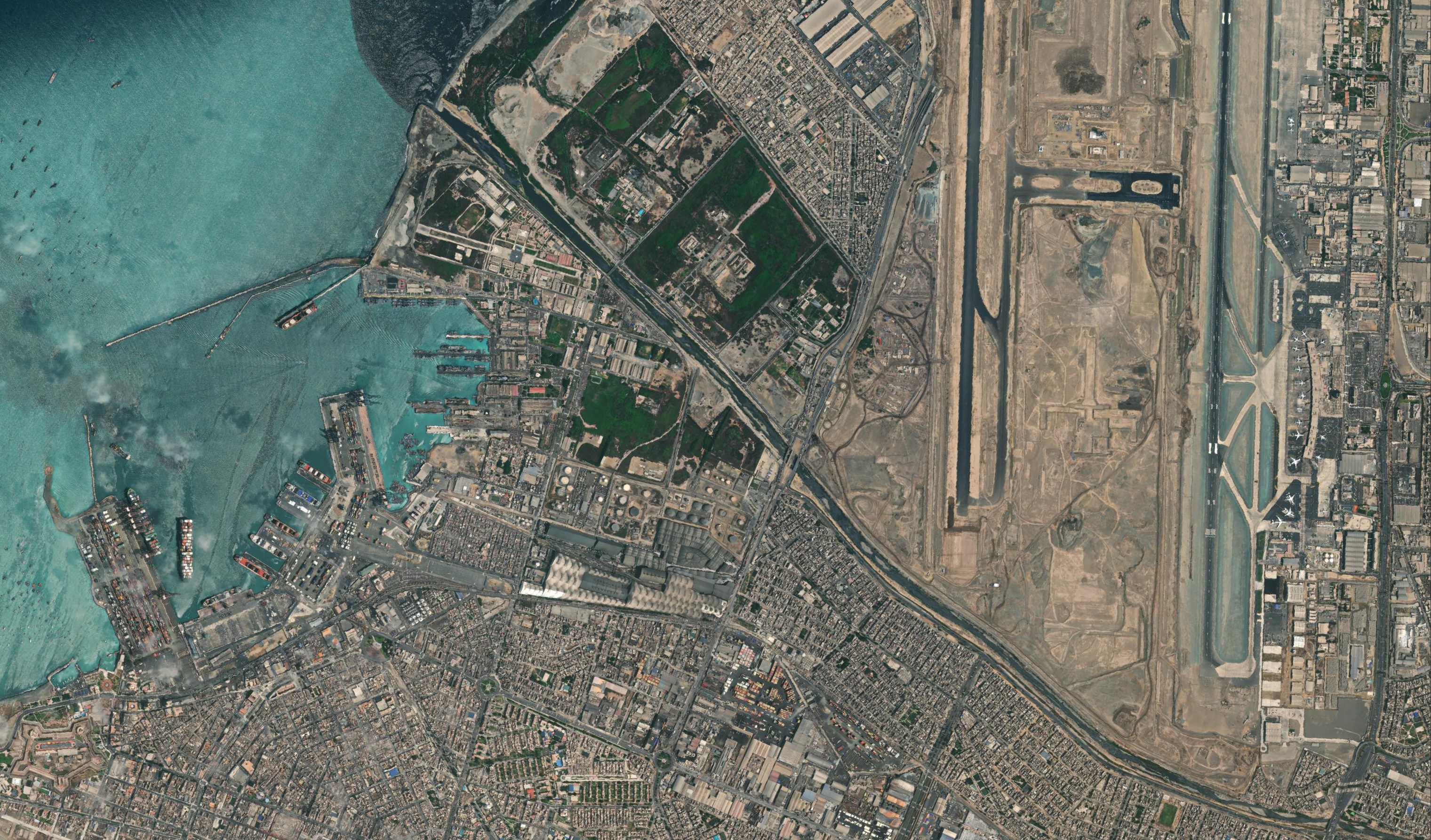
The premium imagery is a real step up from the standard imagery. Below is Lima's Port in the standard offering. The waves on the ocean are visible and there are a few clouds.
Below is the same location in the premium offering. The ocean looks very smooth. Also, the ships and other vehicles are in different locations demonstrating this image wasn't taken at the same time.