In November, I wrote a post on analysing aircraft position telemetry with adsb.lol. At the time, I didn't have a clear way to turn a series of potentially thousands of position points for any one aircraft into a list of flight path trajectories and airport stop-offs.
Since then, I've been downloading adsb.lol's daily feed and in this post, I'll examine the flight routes taken by AirBaltic's YL-AAX Airbus A220-300 aircraft throughout February. I flew on this aircraft on February 24th between Dubai and Riga. I used my memory and notes of the five-hour take-off delay to help validate the enriched dataset in this post.
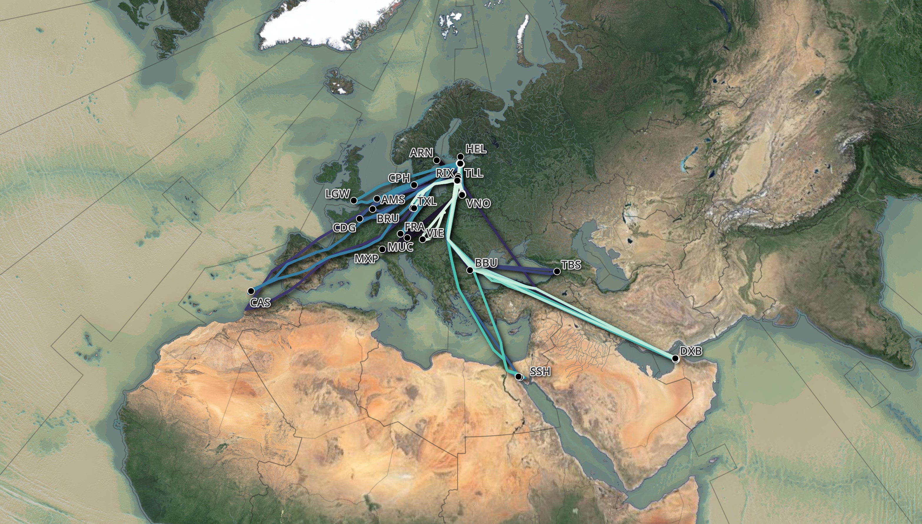
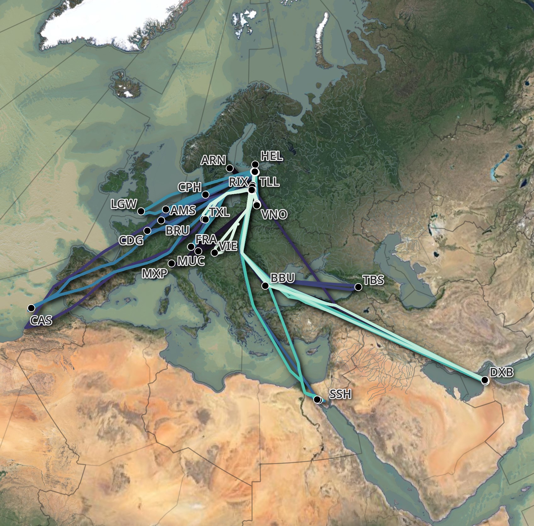
Below is a rendering of the enriched dataset. The darker flight routes are from the beginning of the month and they brighten towards the end of the month.
My Workstation
I'm using a 6 GHz Intel Core i9-14900K CPU. It has 8 performance cores and 16 efficiency cores with a total of 32 threads and 32 MB of L2 cache. It has a liquid cooler attached and is housed in a spacious, full-sized, Cooler Master HAF 700 computer case. I've come across videos on YouTube where people have managed to overclock the i9-14900KF to 9.1 GHz.
The system has 48 GB of DDR5 RAM clocked at 5,200 MHz and a 5th-generation, Crucial T700 4 TB NVMe M.2 SSD which can read at speeds up to 12,400 MB/s. There is a heatsink on the SSD to help keep its temperature down. This is my system's C drive.
There is also an 8 TB mechanical disk that I use to hold GIS datasets. This is my system's F drive.
The system is powered by a 1,200-watt, fully modular, Corsair Power Supply and is sat on an ASRock Z790 Pro RS Motherboard.
I'm running Ubuntu 22 LTS via Microsoft's Ubuntu for Windows on Windows 11 Pro. In case you're wondering why I don't run a Linux-based desktop as my primary work environment, I'm still using an Nvidia GTX 1080 GPU which has better driver support on Windows and I use ArcGIS Pro from time to time which only supports Windows natively.
Installing Prerequisites
I'll first install some dependencies.
$ sudo apt update
$ sudo apt install \
    awscli \
    build-essential \
    cmake \
    python3-virtualenv \
    unzip
Below I'll set up the Python Virtual Environment.
$ virtualenv ~/.adsb
$ source ~/.adsb/bin/activate
$ python -m pip install \
    duckdb \
    flydenity \
    geopandas \
    h3 \
    movingpandas \
    pandas \
    pyarrow \
    rich \
    shapely \
    shpyx \
    typer
Below I'll download and install v0.10.0 of the official binary for DuckDB.
$ cd ~
$ wget -c https://github.com/duckdb/duckdb/releases/download/v0.10.0/duckdb_cli-linux-amd64.zip
$ unzip -j duckdb_cli-linux-amd64.zip
$ chmod +x duckdb
I'll install a few extensions for DuckDB and make sure they load automatically each time I launch the client.
$ ~/duckdb
INSTALL json;
INSTALL parquet;
INSTALL spatial;
$ vi ~/.duckdbrc
.timer on
.width 180
LOAD json;
LOAD parquet;
LOAD spatial;
The maps in this post were rendered with QGIS version 3.36. QGIS is a desktop application that runs on Windows, macOS and Linux. The software is very popular in the geospatial industry and was launched almost 15 million times in May last year.
I used QGIS' Tile+ plugin to add satellite basemaps and Trajectools to turn ADS-B points into trajectories.
Tile+ can be installed from its ZIP distributable.
For Trajectools, I first installed MovingPandas into QGIS' Python Environment. Launch QGIS' Python Console from the Plugins Menu and run the following.
import pip

pip.main(['install', 'scikit-mobility'])
pip.main(['install', 'movingpandas'])
Then after restarting QGIS, find "Trajectools" in the "Manage and Install Plugins" dialog and install it.
I've used Noto Sans for the final map's font.
Downloading ADS-B Data
I've written a script that will download adsb.lol's distributable from two days prior.
$ cat /mnt/f/gis/Global/adsb_lol/download.sh
DATE=`date --date="2 days ago" +"%Y.%m.%d"`
wget -c https://github.com/adsblol/globe_history/releases/download/v$DATE-planes-readsb-prod-0/v$DATE-planes-readsb-prod-0.tar
The above script runs as a daily cronjob. It has been reliable for as long as I've been using it.
$ crontab -l
0 20 * * * bash -c "cd /mnt/f/gis/Global/adsb_lol && bash download.sh"
The downloads are between 1.6 and 1.8 GB for any given day.
$ ls -lht v2024.02.0*
1.8G ... v2024.02.09-planes-readsb-prod-0.tar
1.7G ... v2024.02.08-planes-readsb-prod-0.tar
1.6G ... v2024.02.07-planes-readsb-prod-0.tar
1.6G ... v2024.02.06-planes-readsb-prod-0.tar
1.6G ... v2024.02.05-planes-readsb-prod-0.tar
1.5G ... v2024.02.04-planes-readsb-prod-0.tar
1.6G ... v2024.02.03-planes-readsb-prod-0.tar
1.6G ... v2024.02.02-planes-readsb-prod-0.tar
1.7G ... v2024.02.01-planes-readsb-prod-0.tar
Downloading Natural Earth's Dataset
I'll download Natural Earth's 1:10m scale, version 5.1.2 dataset. It was published in May 2022.
$ mkdir -p /mnt/f/gis/Global/naturalearth

$ for DATASET in cultural physical raster; do
      cd /mnt/f/gis/Global/naturalearth
      aws s3 sync \
            --no-sign-request \
            s3://naturalearth/10m_$DATASET/ \
            10m_$DATASET/

      cd 10m_$DATASET/
      ls *.zip | xargs -n1 -P4 -I% unzip -qn %
  done
The above downloaded three categories of data. In ZIP format, there is 120 MB of physical data (coastlines, lakes, etc..) across 54 ZIP files, 720 MB of cultural data (transport, time zones, populated areas, borders) across 79 ZIP files and 5.6 GB of raster data (relief maps of the earth) across 37 ZIP files.
ADS-B in Parquet Format
I've updated the ADS-B JSON to Parquet enrichment script from the adsb.lol blog post. It can now work across multiple threads with each thread processing an individual tar file. The default pool size is 8 but this can be adjusted.
$ vi enrich.py
#!/usr/bin/env python3
# -*- coding: utf-8 -*-
from   datetime        import datetime
from   glob            import glob
import json
from   multiprocessing import Pool
from   shlex           import quote
import tarfile
import zlib

from   flydenity     import Parser
import h3
from   rich.progress import Progress, track
from   shpyx         import run as execute
import typer


aircraft_keys = set([
    'alert',
    'alt_geom',
    'baro_rate',
    'category',
    'emergency',
    'flight',
    'geom_rate',
    'gva',
    'ias',
    'mach',
    'mag_heading',
    'nac_p',
    'nac_v',
    'nav_altitude_fms',
    'nav_altitude_mcp',
    'nav_heading',
    'nav_modes',
    'nav_qnh',
    'nic',
    'nic_baro',
    'oat',
    'rc',
    'roll',
    'sda',
    'sil',
    'sil_type',
    'spi',
    'squawk',
    'tas',
    'tat',
    'track',
    'track_rate',
    'true_heading',
    'type',
    'version',
    'wd',
    'ws'])

app = typer.Typer(rich_markup_mode='rich')


def gzip_jsonl(filename:str):
    execute('pigz -9 -f %s' % quote(filename))


def process_records(rec, num_recs, out_filename, out_file, source_date):
    parser = Parser() # Aircraft Registration Parser

    # Keep integer form to calculate offset in trace dictionary
    timestamp        = rec['timestamp']
    rec['timestamp'] = str(datetime.utcfromtimestamp(rec['timestamp']))

    if 'year' in rec.keys() and str(rec['year']) == '0000':
        return num_recs, out_filename, out_file

    if 'noRegData' in rec.keys():
        return num_recs, out_filename, out_file

    # Force casing on fields
    rec['icao']      = rec['icao'].lower()

    for key in ('desc', 'r', 't', 'ownOp'):
        if key in rec.keys():
            rec[key]  = rec[key].upper()

    if 'r' in rec.keys():
        reg_details = parser.parse(rec['r'])

        if reg_details:
            rec['reg_details'] = reg_details

    for trace in rec['trace']:
        num_recs = num_recs + 1
        _out_filename = 'traces_%s_%04d.jsonl' % (source_date,
                                                  int(num_recs / 1_000_000))

        if _out_filename != out_filename:
            if out_file:
                out_file.close()

            if out_filename:
                gzip_jsonl(out_filename)

            out_file = open(_out_filename, 'w')
            out_filename = _out_filename

        rec['trace'] = {
            'timestamp': str(datetime.utcfromtimestamp(timestamp +
                                                       trace[0])),
            'lat':                     trace[1],
            'lon':                     trace[2],
            'h3_5':                    h3.geo_to_h3(trace[1],
                                                    trace[2],
                                                    5),
            'altitude':
                trace[3]
                if str(trace[3]).strip().lower() != 'ground'
                else None,
            'ground_speed':            trace[4],
            'track_degrees':           trace[5],
            'flags':                   trace[6],
            'vertical_rate':           trace[7],
            'aircraft':
                {k: trace[8].get(k, None)
                    if trace[8] else None
                 for k in aircraft_keys},
            'source':                  trace[9],
            'geometric_altitude':      trace[10],
            'geometric_vertical_rate': trace[11],
            'indicated_airspeed':      trace[12],
            'roll_angle':              trace[13]}

        out_file.write(json.dumps(rec, sort_keys=True) + '\n')

    return num_recs, out_filename, out_file


def process_file(manifest):
    filename, task = manifest
    num_recs, out_filename, out_file = 0, None, None

    assert '-planes-readsb-prod-0.tar' in filename

    source_date = '20' + filename.split('v20')[-1]\
                                 .split('-')[0]\
                                 .replace('.', '-')

    print(filename)

    with tarfile.open(filename, 'r') as tar:
        for member in tar.getmembers():
            if member.name.endswith('.json'):
                f = tar.extractfile(member)

                if f is not None:
                    rec = json.loads(
                              zlib.decompress(f.read(),
                                              16 + zlib.MAX_WBITS))
                    num_recs, out_filename, out_file = \
                        process_records(rec,
                                        num_recs,
                                        out_filename,
                                        out_file,
                                        source_date)

    if out_file:
        out_file.close()

        if out_filename:
            gzip_jsonl(out_filename)


@app.command()
def main(pattern:str   = 'v*-planes-readsb-prod-0.tar',
         pool_size:int = 8):
    # Get total number of JSON files that will be processed so the
    # progress tracker knows ahead of time.
    total_json_files = {}

    with Progress() as progress:
        task = progress.add_task('Counting JSON Files in each TAR file',
                                 total=len(glob(pattern)))

        for filename in glob(pattern):
            for member in tarfile.open(filename, 'r').getmembers():
                if member.name.endswith('.json'):
                    if filename not in total_json_files.keys():
                        total_json_files[filename] = {'num_recs': 0}

                    total_json_files[filename]['num_recs'] = \
                        total_json_files[filename]['num_recs'] + 1

            progress.update(task, advance=1)


    # Process every JSON file in each .tar file.
    # WIP: Find a way to share the progress bar across threads
    pool = Pool(pool_size)
    payload = [(k, total_json_files[k]['task'])
               for k in total_json_files.keys()]
    pool.map(process_file, payload)


if __name__ == "__main__":
    app()
A glob pattern can be used to isolate the script's workload to a handful of files. Otherwise, it'll try to match to adsb.lol's file naming convention.
$ python enrich.py
I haven't found a way to share the progress bar across multiple threads so when the pool is executing, progress is indicated by the file name of each tar file being printed as its first opened.
For any given day, there will be ~45 Parquet files generated. Each Parquet file contains one million records for that day's flight traces. This partitioning is done to ensure DuckDB doesn't run out of memory when processing each file on a RAM-constrained system.
My main workstation has 48 GB of RAM but I've also run this script on a Steam Deck with 16 GB of RAM and a MacBook Pro with 8 GB of RAM without issue.
The resulting Parquet files are around 45 MB each. Here are the file sizes of a few of them.
$ ls -lht traces_2024-02-29_003*.pq
45M ... traces_2024-02-29_0039.pq
44M ... traces_2024-02-29_0038.pq
45M ... traces_2024-02-29_0037.pq
45M ... traces_2024-02-29_0036.pq
45M ... traces_2024-02-29_0035.pq
45M ... traces_2024-02-29_0034.pq
45M ... traces_2024-02-29_0033.pq
45M ... traces_2024-02-29_0032.pq
45M ... traces_2024-02-29_0031.pq
45M ... traces_2024-02-29_0030.pq
There are 1,186,616,930 records in total for February.
Better Compression
This is an optional step but if you're archiving the Parquet files or sharing them with a large number of people, the file sizes can be reduced from ~45 MB to around ~13 MB each. This is done by a combination of sorting and stronger compression.
I'll use a Parquet debugging tool I've been working on to see how much space each column takes up in one of the Parquet files.
$ git clone https://github.com/marklit/pqview \
    ~/pqview

$ virtualenv ~/.pqview
$ source ~/.pqview/bin/activate
$ python3 -m pip install \
          -r ~/pqview/requirements.txt
$ python3 ~/pqview/main.py \
    types --html \
    traces_2024-02-29_0045.pq \
    > traces_2024-02-29_0045.html
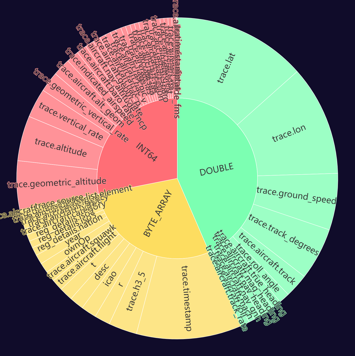
The trace.lon field is one of the largest in the Parquet file. It often has the largest number of unique values compared to any other column as well. ZStandard's compression efficiency is sensitive to sorting so this column being the sort key should offer the smallest resulting files.
Below I'll patch DuckDB's source code changing the default ZStandard compression level from 3 to 22.
$ git clone https://github.com/duckdb/duckdb.git ~/duckdb_source

$ cd ~/duckdb_source
$ mkdir -p build/release
Below is where the default value is stored.
$ grep -R 'define ZSTD_CLEVEL_DEFAULT' third_party/zstd/
third_party/zstd/include/zstd.h:# define ZSTD_CLEVEL_DEFAULT 3
I changed the above to 22.
diff --git a/third_party/zstd/include/zstd.h b/third_party/zstd/include/zstd.h
index ade94c2d5c..80d4b560a9 100644
--- a/third_party/zstd/include/zstd.h
+++ b/third_party/zstd/include/zstd.h
@@ -84,7 +84,7 @@ ZSTDLIB_API const char* ZSTD_versionString(void);   /* requires v1.3.0+ */
  *  Default constant
  ***************************************/
 #ifndef ZSTD_CLEVEL_DEFAULT
-#  define ZSTD_CLEVEL_DEFAULT 3
+#  define ZSTD_CLEVEL_DEFAULT 22
 #endif

/* *************************************
Below I'll compile the code and launch the resulting binary.
$ cmake \
    ./CMakeLists.txt \
    -DCMAKE_BUILD_TYPE=RelWithDebInfo \
    -DEXTENSION_STATIC_BUILD=1 \
    -DBUILD_PARQUET_EXTENSION=1 \
    -B build/release

$ CMAKE_BUILD_PARALLEL_LEVEL=$(nproc) \
    cmake --build build/release
$ ~/duckdb_source/build/release/duckdb -unsigned
This binary needs to use the Parquet extension that it was compiled with.
INSTALL '/home/mark/duckdb_source/build/release/extension/parquet/parquet.duckdb_extension';
LOAD parquet;
The re-compressed Parquet file is 12,888,833 bytes. It can be read without issue by the officially distributed versions of DuckDB, not just the patched version above.
COPY(
    SELECT   *
    FROM     READ_PARQUET('/mnt/f/gis/Global/adsb_lol/traces_2024-02-29_0045.pq')
    ORDER BY trace.lon
) TO 'test.zstd.22.pq' (FORMAT 'PARQUET',
                        CODEC  'ZSTD',
                        ROW_GROUP_SIZE 15000);
AirBaltic's Fleet
Normally the ownOp field in each trace record will be populated with an Airline's brand like 'DELTA AIR LINES INC ' or 'WESTJET'. AirBaltic's traces don't populate this field.
They only fly the Airbus A220-300 (identified as BCS3 in the traces) and all 47 of their aircraft are registered in Latvia. They are also the only Latvian owner of this type of aircraft. I'll use these details to find all of their unique registration numbers in this dataset.
$ ~/duckdb working.duckdb
.maxrows 100

SELECT DISTINCT r
FROM            READ_PARQUET('/mnt/f/gis/Global/adsb_lol/traces*.pq')
WHERE           reg_details.nation = 'Latvia'
AND             t = 'BCS3'
ORDER BY        1;
┌─────────┐
│    r    │
│ varchar │
├─────────┤
│ YL-AAO  │
│ YL-AAP  │
│ YL-AAQ  │
│ YL-AAR  │
│ YL-AAS  │
│ YL-AAT  │
│ YL-AAU  │
│ YL-AAV  │
│ YL-AAW  │
│ YL-AAX  │
│ YL-AAY  │
│ YL-AAZ  │
│ YL-ABA  │
│ YL-ABB  │
│ YL-ABD  │
│ YL-ABE  │
│ YL-ABF  │
│ YL-ABG  │
│ YL-ABH  │
│ YL-ABI  │
│ YL-ABJ  │
│ YL-ABK  │
│ YL-ABL  │
│ YL-ABM  │
│ YL-ABN  │
│ YL-ABO  │
│ YL-ABP  │
│ YL-ABQ  │
│ YL-ABR  │
│ YL-ABS  │
│ YL-ABT  │
│ YL-CSA  │
│ YL-CSB  │
│ YL-CSC  │
│ YL-CSD  │
│ YL-CSF  │
│ YL-CSI  │
│ YL-CSJ  │
│ YL-CSK  │
│ YL-CSL  │
│ YL-CSM  │
│ YL-CSN  │
├─────────┤
│ 42 rows │
└─────────┘
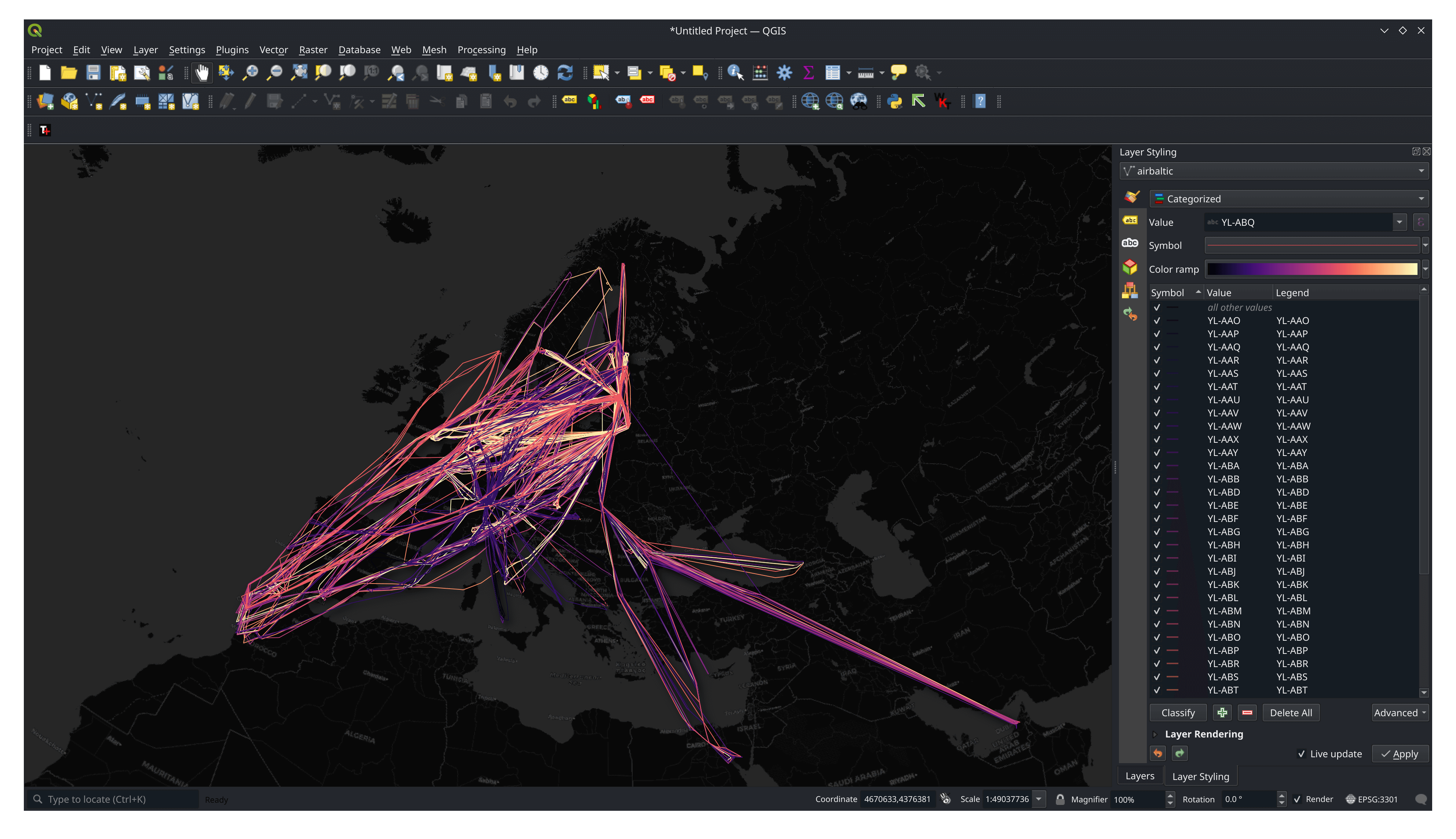
I came across all but five of their aircraft. Below is a rendering of their movements in February. Each aircraft has its own unique colour. I'm still trying to find a way to do fleet movement generalisation.
Detecting Stop-offs
Below I'll take all the positions reported for AirBaltic's YL-AAX aircraft and detect its routes and stop-offs.
$ source ~/.adsb/bin/activate
$ python3
from   datetime     import timedelta
import json

import duckdb
import geopandas    as gpd
import movingpandas as mpd
import pandas       as pd
from   shapely      import Point
from   shapely.ops  import nearest_points
from   shapely.wkt  import loads


con = duckdb.connect(database=':memory:')
df = con.sql("""INSTALL spatial;
                LOAD    spatial;

                SELECT ST_ASTEXT(ST_POINT(trace.lon, trace.lat)) AS geom,
                       trace."timestamp"::TIMESTAMP   AS observed_at,
                       icao,
                       r,
                       t,
                       ownOp,
                       trace.altitude,
                       trace.flags,
                       trace.geometric_altitude,
                       trace.geometric_vertical_rate,
                       trace.ground_speed,
                       trace.h3_5,
                       trace.indicated_airspeed,
                       trace.roll_angle,
                       trace.source,
                       trace.track_degrees,
                       trace.vertical_rate
                FROM   READ_PARQUET('traces*.pq')
                WHERE  r = 'YL-AAX'""").to_df()

df['geom']        = df['geom'].apply(lambda x: loads(x))
df['observed_at'] = pd.to_datetime(df['observed_at'],
                                   format='mixed')

traj_collection = \
    mpd.TrajectoryCollection(
            gpd.GeoDataFrame(df,
                             crs='4326',
                             geometry='geom'),
            'r',
            t='observed_at')

detector = mpd.TrajectoryStopDetector(traj_collection)

stop_time_ranges = \
    detector.get_stop_time_ranges(
        min_duration=timedelta(minutes=20),
        max_diameter=100_000)

stop_points = \
    detector.get_stop_points(
        min_duration=timedelta(minutes=20),
        max_diameter=100_000)
The stop points aren't always right on an airport's runway and can sometimes be 40 or 50 KM away from the airport itself. Below are the stop points for Dubai in February.
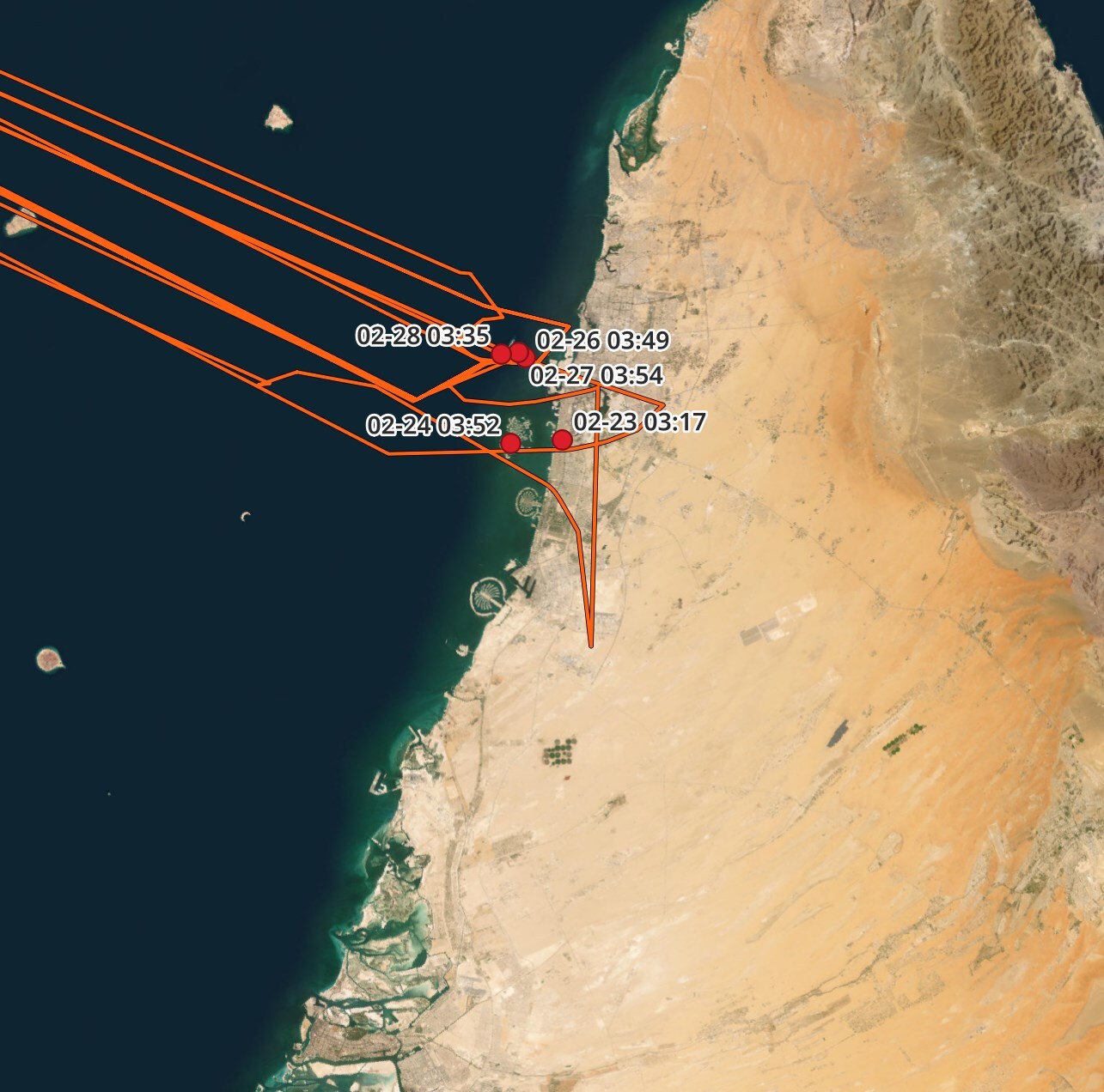
The coverage for the Middle East in this dataset is very sparse and there are almost no traces in the Gulf 50 KM beyond Dubai's International Airport.
There is one trace flying south of the airport in the above rendering that abruptly turns around. This was my aircraft diverting to another Airport due to fog. Its ADS-B signal was outside the range of adsb.lol's network of receivers so its journey to Al Ain Airport isn't fully visible in this dataset.
These are the stop points for Tallinn in February. None are within 30 KM of Tallinn's airport. It could very well be that some adjust settings for MovingPandas would place these points closer to where the aircraft was on the ground.
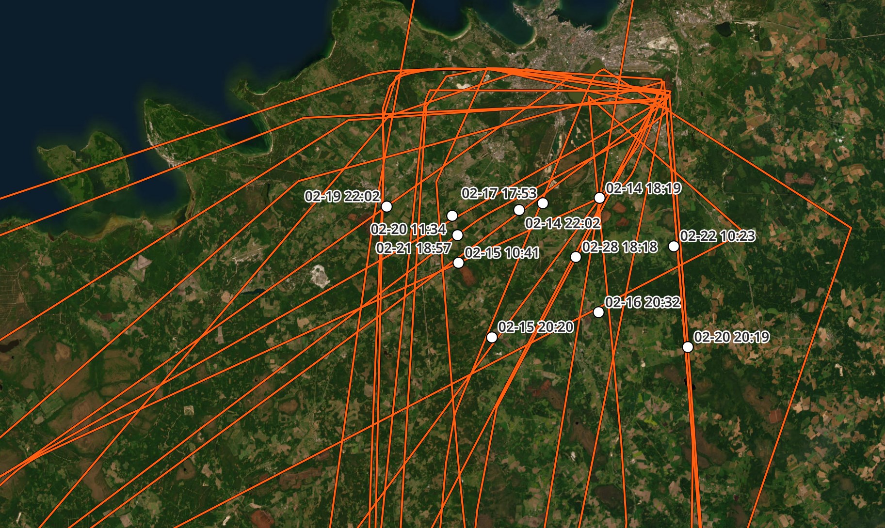
I'll try and quantise / snap each landing point to its nearest airport. I usually see 95%+ accuracy with this code.
airports_df = \
    gpd.read_file('/mnt/f/gis/Global/natural_earth/'
                  '10m_cultural/ne_10m_airports/ne_10m_airports.shp')

stops = json.loads(stop_points['geometry'].to_json())

for num, feature in enumerate(stops['features']):
    nearest_point = \
        nearest_points(Point(feature['geometry']['coordinates']),
                       airports_df.unary_union)

    stops['features'][num]['properties'] = {
        'nearest_airport':
            json.loads(airports_df.loc[airports_df["geometry"] ==
                        nearest_point[1]].to_json())}

open('stops-airports.geojson', 'w').write(json.dumps(stops))
The above found 69 stops for this Aircraft in February.
$ jq -S '.features|length' stops-airports.geojson
69
Below is a GeoJSON record for the first of these stops.
$ jq -S .features[0] stops-airports.geojson
{
  "bbox": [
    23.77087,
    56.954132,
    23.77087,
    56.954132
  ],
  "geometry": {
    "coordinates": [
      23.77087,
      56.954132
    ],
    "type": "Point"
  },
  "id": "YL-AAX_2024-02-02 13:38:15.200000",
  "properties": {
    "nearest_airport": {
      "features": [
        {
          "geometry": {
            "coordinates": [
              23.979379111699508,
              56.922003878609694
            ],
            "type": "Point"
          },
          "id": "731",
          "properties": {
            "abbrev": "RIX",
            "comments": null,
            "featurecla": "Airport",
            "gps_code": "EVRA",
            "iata_code": "RIX",
            "location": "terminal",
            "name": "Riga",
            "name_ar": "مطار ريغا الدولي",
            "name_bn": null,
            "name_de": "Flughafen Riga",
            "name_el": null,
            "name_en": "Riga International Airport",
            "name_es": "Aeropuerto Internacional de Riga",
            "name_fa": "فرودگاه بینالمللی ریگا",
            "name_fr": "aéroport international de Riga",
            "name_he": "נמל התעופה הבינלאומי ריגה",
            "name_hi": null,
            "name_hu": "Rigai nemzetközi repülőtér",
            "name_id": "Bandar Udara Internasional Riga",
            "name_it": "Aeroporto Internazionale di Riga",
            "name_ja": "リガ国際空港",
            "name_ko": "리가 국제공항",
            "name_nl": "Luchthaven Riga",
            "name_pl": "Port lotniczy Ryga",
            "name_pt": "Aeroporto Internacional de Riga",
            "name_ru": "Рига",
            "name_sv": "Riga flygplats",
            "name_tr": "Riga Uluslararası Havalimanı",
            "name_uk": "Рига",
            "name_ur": null,
            "name_vi": "Sân bay quốc tế Riga",
            "name_zh": "里加国际机场",
            "name_zht": "里加國際機場",
            "natlscale": 50,
            "ne_id": 1159125897,
            "scalerank": 4,
            "type": "major",
            "wdid_score": 4,
            "wikidataid": "Q505421",
            "wikipedia": "http://en.wikipedia.org/wiki/Riga_International_Airport"
          },
          "type": "Feature"
        }
      ],
      "type": "FeatureCollection"
    }
  },
  "type": "Feature"
}
I printed out the stops for the month and examined the flights around my February 24th flight with this aircraft.
last_date = None

for x in stops['features']:
    _, ts      = x['id'].split('_')
    this_date  = ts.split(' ')[0]
    short_time = ts.split(' ')[1].split('.')[0][:5]

    if last_date != this_date:
        print()
        last_date = this_date
    elif not last_date:
        last_date = this_date

    print(this_date,
          short_time,
          x['properties']
           ['nearest_airport']
           ['features']
           [0]
           ['properties']
           ['name'])
...
2024-02-23 03:17 Dubai Int'l
2024-02-23 13:24 Riga
2024-02-23 17:59 Berlin-Tegel Int'l
2024-02-23 20:12 Riga

2024-02-24 03:52 Dubai Int'l
2024-02-24 17:15 Riga

2024-02-25 10:17 Sharm el-Sheikh Int'l
2024-02-25 16:14 Riga
2024-02-25 19:46 Riga

2024-02-26 03:49 Dubai Int'l
2024-02-26 13:07 Riga

2024-02-27 03:54 Dubai Int'l
2024-02-27 12:33 Riga
...
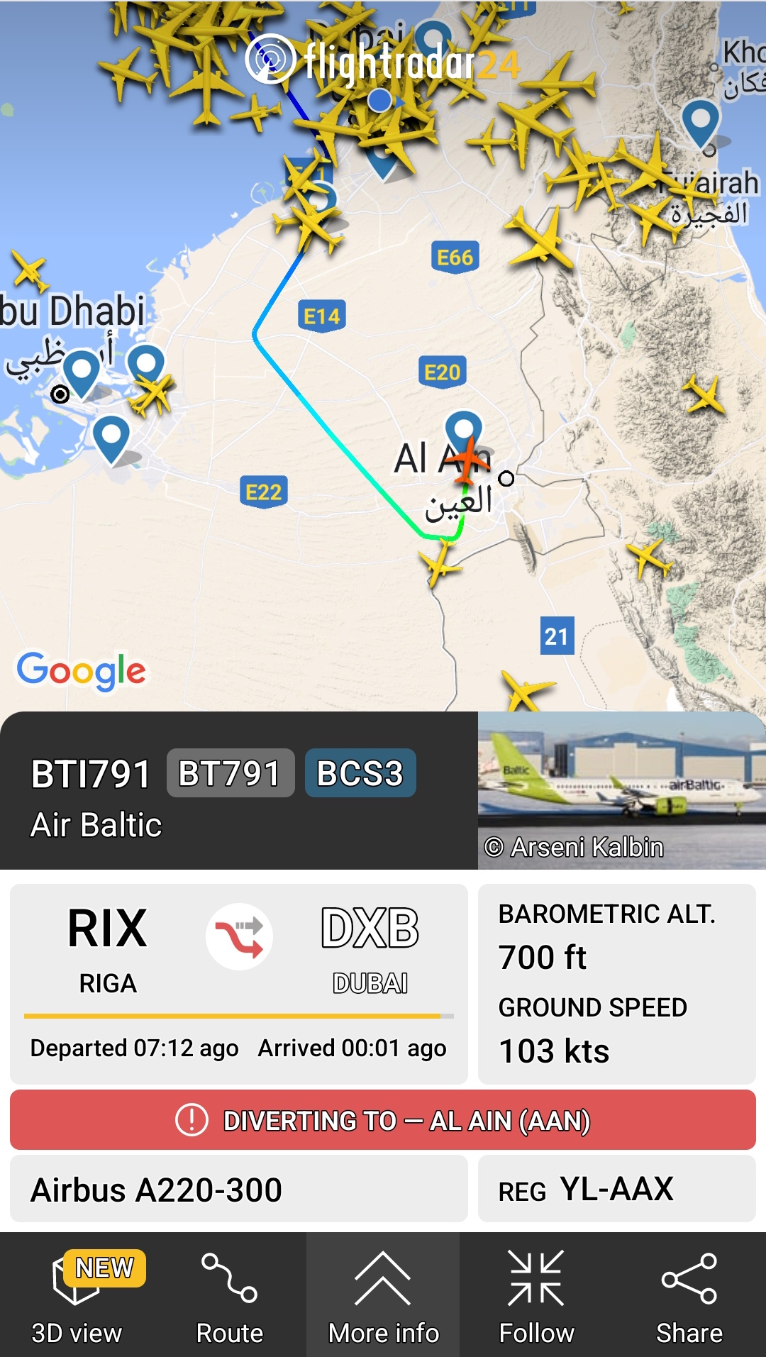
Normally, the aircraft will first be seen flying into Dubai around 03:30 UTC which is 7:30 AM local time. Below is FlightRadar24's tracking of the Aircraft after it diverted from Dubai International to Al Ain Airport.
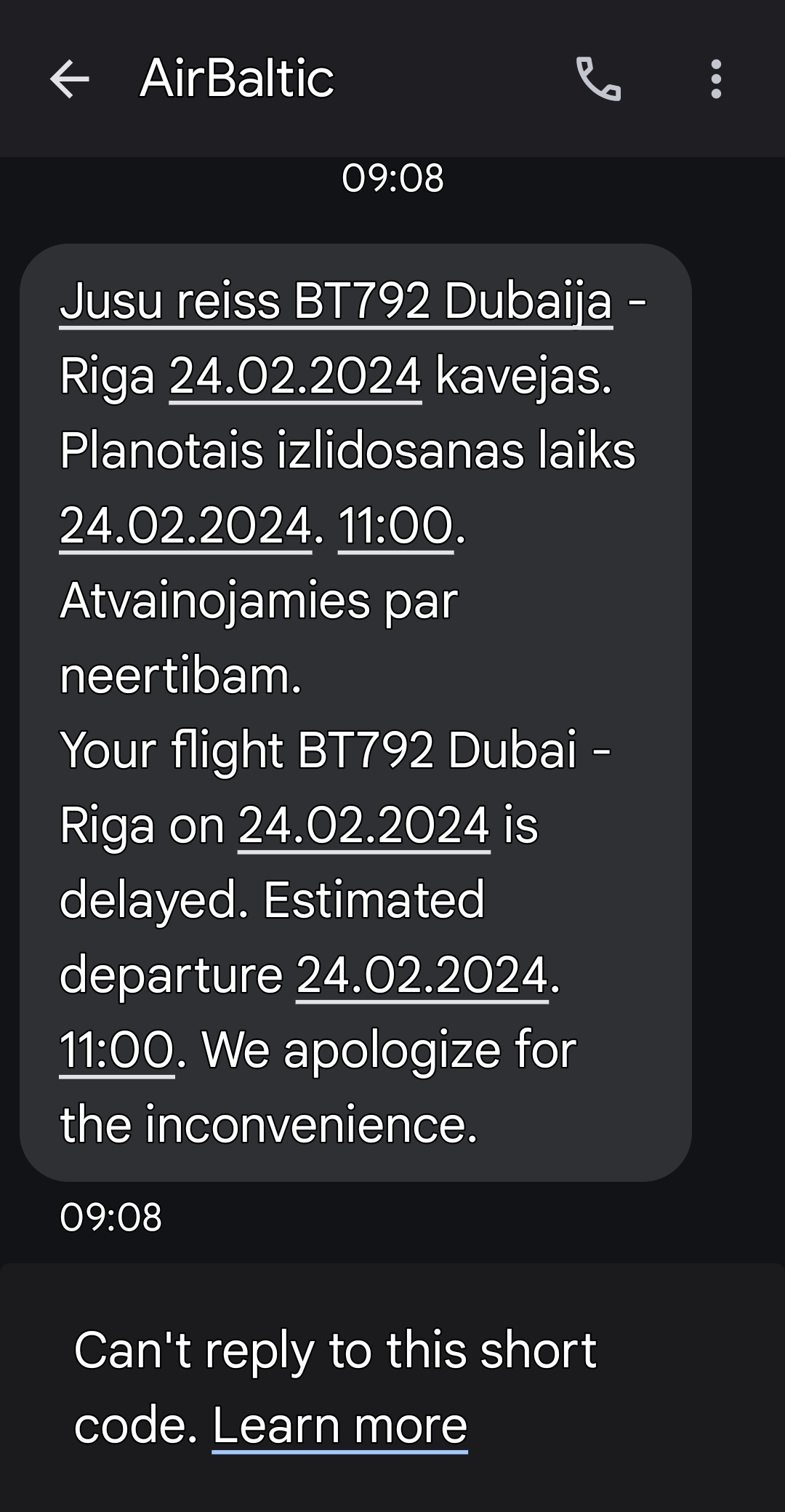
Below is an SMS from AirBaltic shortly after the diversion was announced on FlightRadar24.
That flight normally will later then be seen in Riga around 13:15 UTC. My flight was delayed due to fog in Dubai so our flight reached Riga around 17:15 UTC.
Exporting Aircraft Traces
I'll export the positions of this Aircraft for February to a GeoPackage File.
$ ~/duckdb working.duckdb
COPY(
    SELECT   ST_POINT(trace.lon, trace.lat) AS geom,
             trace."timestamp"::TIMESTAMP   AS observed_at,
             icao,
             r,
             t,
             ownOp,
             trace.altitude,
             trace.flags,
             trace.geometric_altitude,
             trace.geometric_vertical_rate,
             trace.ground_speed,
             trace.h3_5,
             trace.indicated_airspeed,
             trace.roll_angle
             trace.source,
             trace.track_degrees,
             trace.vertical_rate
    FROM     READ_PARQUET('traces*.pq')
    WHERE    r = 'YL-AAX'
    ORDER BY trace.timestamp
) TO 'YL-AAX.gpkg'
  WITH (FORMAT GDAL,
        DRIVER 'GPKG',
        LAYER_CREATION_OPTIONS 'WRITE_BBOX=YES');
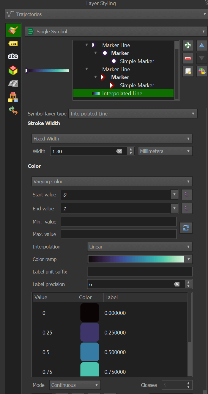
I'll then open it in its own layer in QGIS and use Trajectools to generate the trajectories. This will result in a trajectory layer with an interpolated line that is easy to style.
Make sure this layer has a projection of EPSG:4326 before running Trajectools.
Plotting Routes on a Map
These are the layers in my QGIS project.
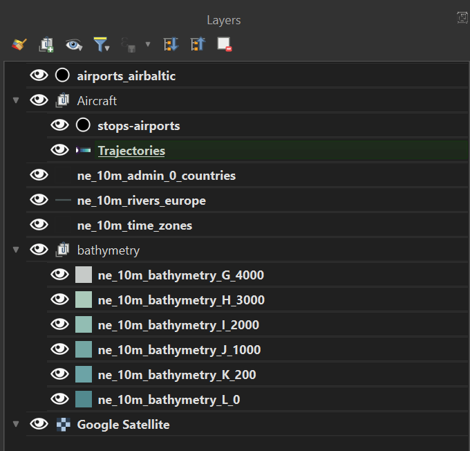
The bottom layer is a Google Satellite Basemap that I added with the Tile+ plugin.
Above that, I added Natural Earth's Bathymetry layers from sea level till 4000 meters. They've been coloured #52898e, #6ca3a6, #74a6a3, #92bdb3, #abcaba and #c6cac8 respectively. These layers are rendered as a group with a subtractive blending mode.
Then I have Natural Earth's Timezone dataset with a 0.5-point stroke coloured #232323.
Then I have Natural Earth's European Rivers dataset with a 0.26-point stroke coloured #667b7c.
Then I have Natural Earth's Admin-0 Countries dataset with a 0.5-point stroke coloured #232323.
The labels use Noto Sans SemiBold with a white text buffer.
The trajectories interpolated line uses the Mako gradient preset.
I added in the 69-record stop points GeoJSON file on top of the existing trajectories layer. I first tried to label the airports using the landing points but because every landing was in a slightly different location, duplicate labels appeared. 45 minutes of Googling and experimentation with QGIS' labelling engine wouldn't get rid of these duplicates either. I ended up creating a new vector layer and I manually plotted each airport and its 3-letter code by hand.
The map's projection has been set to EPSG:3301.