Automatic Dependent Surveillance-Broadcast (ADS-B) is an aircraft tracking system. Nearly all aircraft periodically broadcast their details, position and other metrics over radio waves that can be picked up by anyone with an ADS-B receiver on the ground. A modest receiver and antenna can receive messages from planes that are 10s or even 100s of KM away.
ADS-B kits for Raspberry Pis have been popular for almost a decade now and sites like FlightRadar24 receive ADS-B feeds from 10s of thousands of volunteers around the globe every day. These volunteer-collected feeds power most flight-tracking websites.
Some feed aggregators provide free access to analyse their historical data but often require you to register and potentially participate in submitting ADS-B data as well.
I recently came across ADSB.lol which publishes a registration-free feed every day to GitHub of the previous day's aircraft flight traces. The project has been running since March and 38 million aircraft traces were collected on Sunday alone. The project is the work of Katia Esposito, a Site Reliability Engineer based in the Netherlands.
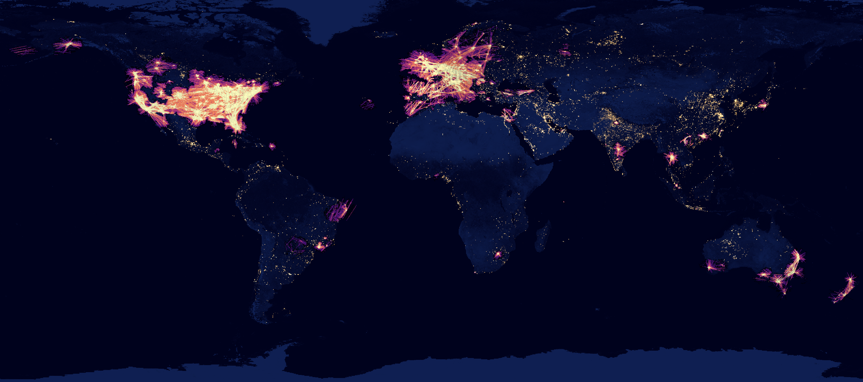
Below is a heatmap of the aircraft positions seen in Sunday's feed. Though there are gaps in the data that an expanded feeder network will hopefully plug, this is still a valuable dataset as it has no barriers to entry and can be analysed with little effort.
In this post, I'll walk through converting a day's worth of data into Parquet and analysing it with DuckDB and QGIS.
Installing Prerequisites
The following was run on Ubuntu for Windows which is based on Ubuntu 20.04 LTS. The system is powered by an Intel Core i5 4670K running at 3.40 GHz and has 32 GB of RAM. The primary partition is a 2 TB Samsung 870 QVO SSD.
I'll be using Python to enrich and analyse the trace files in this post.
$ sudo apt update
$ sudo apt install \
    jq \
    python3-pip \
    python3-virtualenv
$ virtualenv ~/.adsb
$ source ~/.adsb/bin/activate
$ python -m pip install \
    flydenity \
    geopandas \
    h3 \
    movingpandas \
    pandas \
    pyarrow \
    rich \
    shapely \
    typer
I'll also use DuckDB, along with its JSON, Parquet and Spatial extensions, in this post.
$ cd ~
$ wget -c https://github.com/duckdb/duckdb/releases/download/v0.9.2/duckdb_cli-linux-amd64.zip
$ unzip -j duckdb_cli-linux-amd64.zip
$ chmod +x duckdb
$ ~/duckdb
INSTALL json;
INSTALL parquet;
INSTALL spatial;
I'll set up DuckDB to load all these extensions each time it launches.
$ vi ~/.duckdbrc
.timer on
.width 180
LOAD json;
LOAD parquet;
LOAD spatial;
The maps in this post were rendered with QGIS version 3.34. QGIS is a desktop application that runs on Windows, macOS and Linux. I used NASA's Earth at Night basemap in every map as well.
Downloading Flight Traces
I'll download and extract Sunday's tarball.
$ wget https://github.com/adsblol/globe_history/releases/download/v2023.11.19-planes-readsb-prod-0/v2023.11.19-planes-readsb-prod-0.tar
$ mkdir 2023-11-19
$ cd 2023-11-19
$ tar -xf ../v2023.11.19-planes-readsb-prod-0.tar
The 1.6 GB tar file contains 1.1 GB of GZIP-compressed JSON across 47K files. There are also 418 MB of heatmaps and 309 KB of Airborne Collision Avoidance System (ACAS) data.
Below are the root elements of a trace file.
$ gunzip -c traces/01/trace_full_c03001.json \
    | jq -S 'del(.trace)'
{
  "dbFlags": 0,
  "desc": "BOEING 737 MAX 8",
  "icao": "c03001",
  "ownOp": "Air Canada",
  "r": "C-FSEQ",
  "t": "B38M",
  "timestamp": 1700352000,
  "year": "2018"
}
This trace file has 1,610 traces within it.
$ gunzip -c traces/01/trace_full_c03001.json \
    | jq -S '.trace|length'
1610
Below is one of the traces.
$ gunzip -c traces/01/trace_full_c03001.json \
    | jq -S '.trace[10]'
[
  4472.99,
  26.990753,
  -110.817641,
  36000,
  405.8,
  309.3,
  0,
  0,
  {
    "alert": 0,
    "alt_geom": 38025,
    "baro_rate": 0,
    "category": "A3",
    "flight": "ACA971  ",
    "gva": 2,
    "nac_p": 10,
    "nac_v": 2,
    "nav_altitude_mcp": 36000,
    "nav_heading": 293.91,
    "nav_qnh": 1013.6,
    "nic": 8,
    "nic_baro": 1,
    "rc": 186,
    "sda": 2,
    "sil": 3,
    "sil_type": "perhour",
    "spi": 0,
    "track": 309.3,
    "type": "adsb_icao",
    "version": 2
  },
  "adsb_icao",
  38025,
  null,
  null,
  null
]
Where Planes Flew
Below I'll build a heatmap of where aircraft reported their positions throughout Sunday.
$ python3
import gzip
import json
from   glob import glob

from   h3 import geo_to_h3, \
                 h3_to_geo_boundary as get_poly
There are around ~6.5 GB of JSON data across the 47K trace files.
print(sum([len(gzip.open(x).read())
           for x in glob('traces/*/*.json')]))
I'll generate the H3 zoom level 5 cell values for each latitude and longitude pair found within each trace.
with open('h3_5s.txt', 'w') as f:
    for filename in glob('traces/*/*.json'):
        rec = json.loads(gzip.open(filename).read())

        f.write('\n'.join([geo_to_h3(trace[1],
                                     trace[2],
                                     5)
                           for trace in rec['trace']]))
I'll then get a count for each unique H3 value.
$ sort h3_5s.txt \
    | uniq -c \
    > h3_5s_agg.txt
I'll generate a CSV file with the count and geometry for each H3 cell. The geometry will be expressed in Well-Known Text (WKT) format.
def h3_to_wkt(h3_hex:str):
    return 'POLYGON((%s))' % \
               ', '.join(['%f %f' % (lon, lat)
                          for lon, lat in get_poly(h3_hex,
                                                   geo_json=True)])

with open('h3_5s_agg.csv', 'w') as f:
    f.write('wkt,num_observations\n')

    for line in open('h3_5s_agg.txt'):
        count, h3_9 = line.strip().split(' ')
        count = int(count)
        h3_9 = h3_9.strip()

        if len(h3_9) == 15:
            f.write('"%s",%d\n' % (h3_to_wkt(h3_9), count))
Below is the header and the first record of the CSV file.
$ head -n2 h3_5s_agg.csv
wkt,num_observations
"POLYGON((20.534114 70.247680, 20.673926 70.302878, 20.572140 70.373370, 20.329325 70.388360, 20.190070 70.332817, 20.293064 70.262629, 20.534114 70.247680))",1
This is the heatmap of aircraft positions seen across the globe. Yellow indicates where the most aircraft were seen.
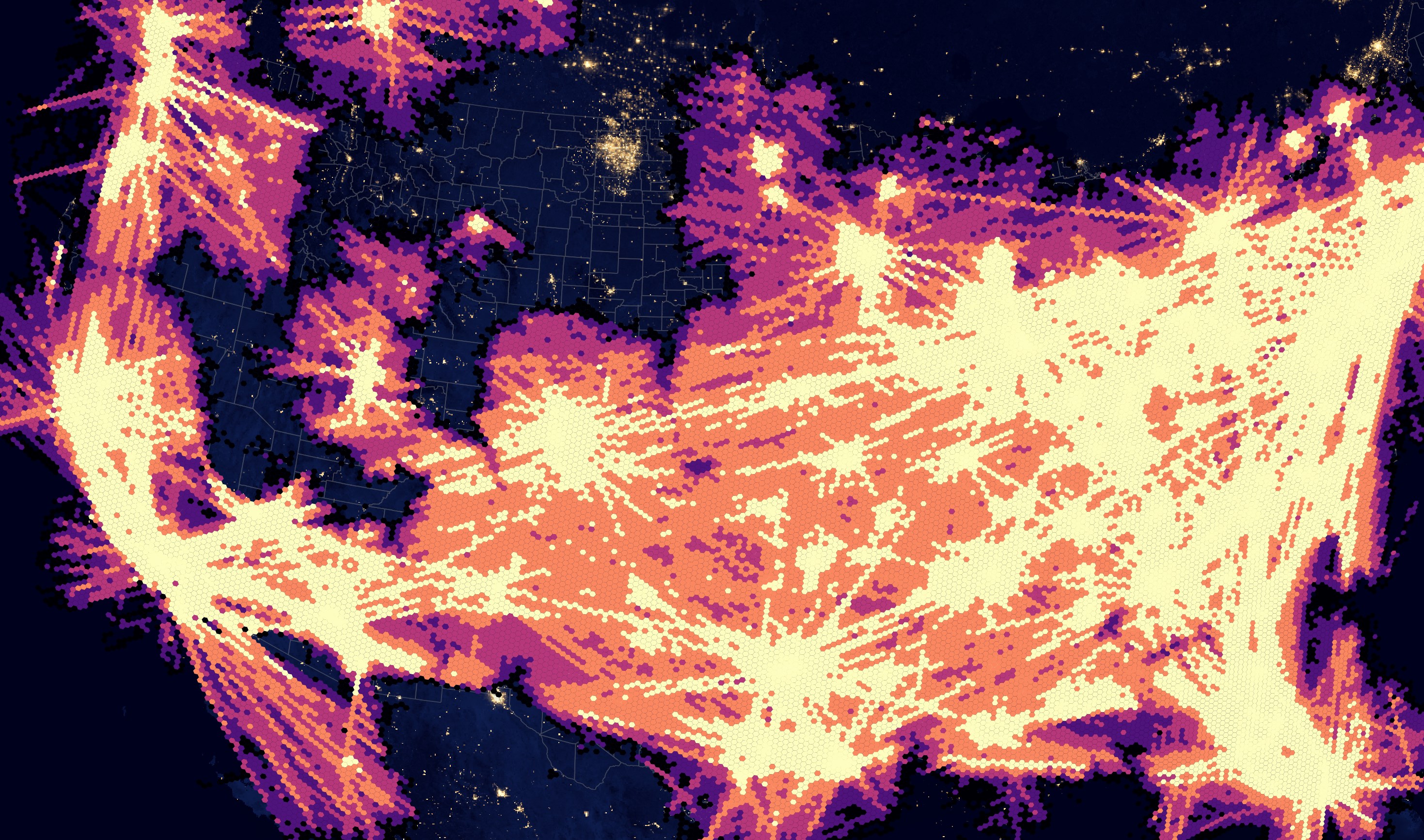
In the US, the most common positions line up with the US' population density hotspots.
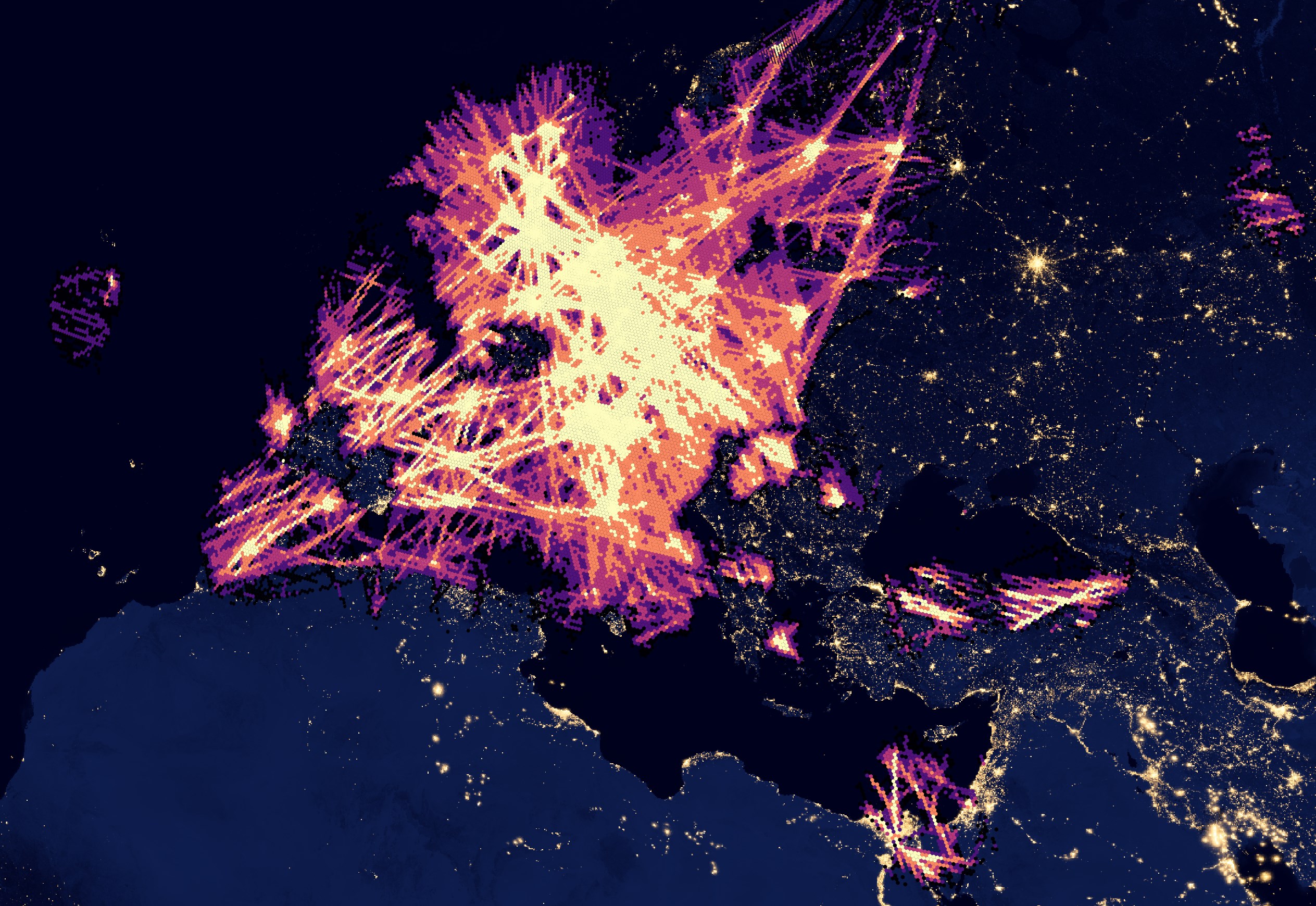
Much of Europe is covered as well but there are notable gaps across Russia and the Canary Islands.
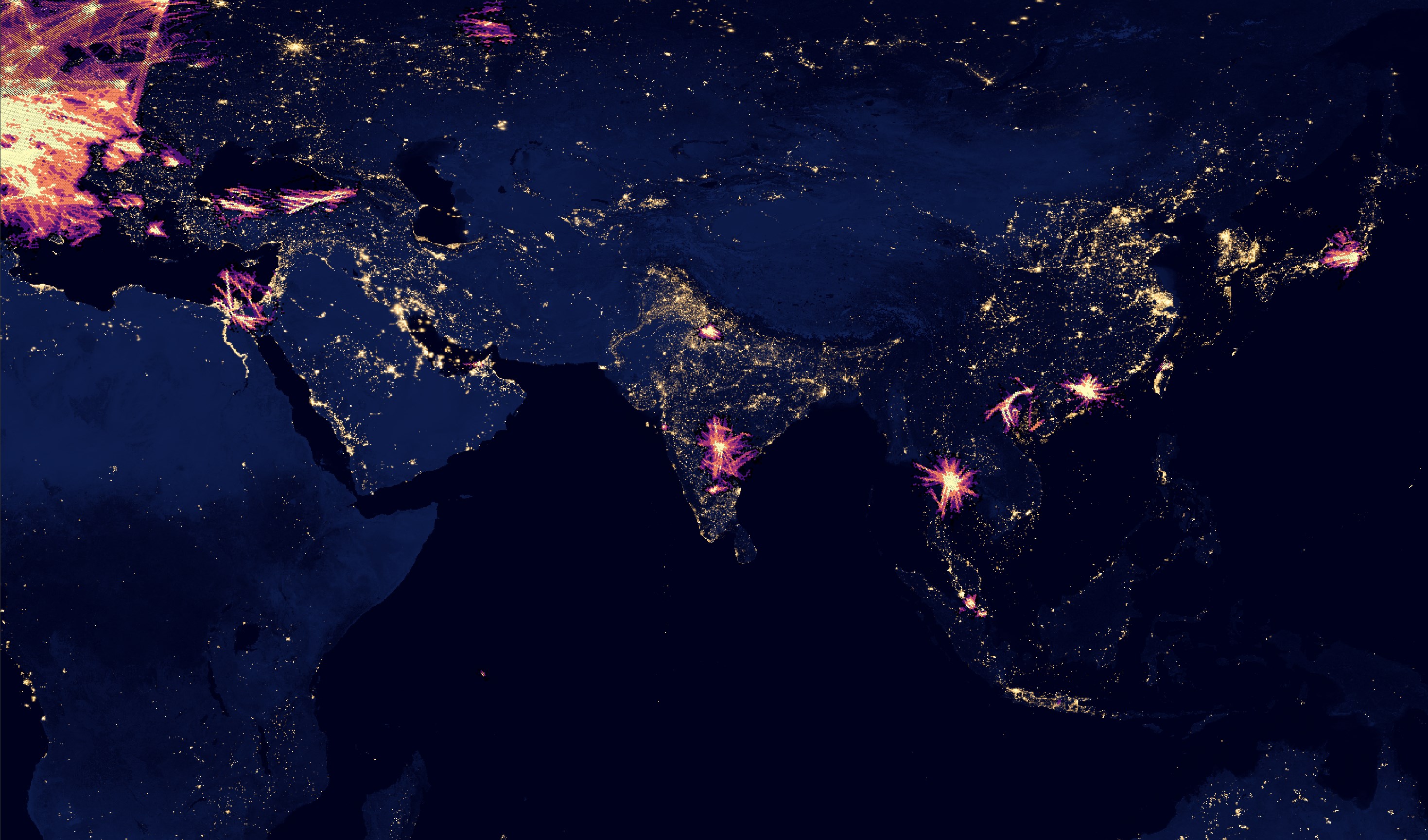
In the Gulf, there are almost no aircraft positions recorded outside of Dubai even though the route between the UAE and Europe is one of the busiest.
India, Thailand and Japan all have clusters but the heatmap is nowhere near representative of the actual number of aircraft that would have flown over these countries on Sunday.
Creating Enriched Parquet Files
I'll enrich the original JSON trace files and store the resulting data in ~1M-row JSONL files.
$ python3
from   datetime import datetime
from   glob import glob
import gzip
import json

from   flydenity import Parser
import h3
from   rich.progress import track


aircraft_keys = set([
    'alert',
    'alt_geom',
    'baro_rate',
    'category',
    'emergency',
    'flight',
    'geom_rate',
    'gva',
    'ias',
    'mach',
    'mag_heading',
    'nac_p',
    'nac_v',
    'nav_altitude_fms',
    'nav_altitude_mcp',
    'nav_heading',
    'nav_modes',
    'nav_qnh',
    'nic',
    'nic_baro',
    'oat',
    'rc',
    'roll',
    'sda',
    'sil',
    'sil_type',
    'spi',
    'squawk',
    'tas',
    'tat',
    'track',
    'track_rate',
    'true_heading',
    'type',
    'version',
    'wd',
    'ws'])

parser = Parser() # Aircraft Registration Parser
out_filename, out_file, num_recs = None, None, 0
json_files = [x for x in glob('traces/*/*.json')]

for filename in track(json_files, 'JSON Enrichment..'):
    rec = json.loads(gzip.open(filename).read())

    # Keep integer form to calculate offset in trace dictionary
    timestamp        = rec['timestamp']
    rec['timestamp'] = str(datetime.utcfromtimestamp(rec['timestamp']))

    if 'year' in rec.keys() and str(rec['year']) == '0000':
        continue

    if 'noRegData' in rec.keys():
        continue

    # Force casing on fields
    rec['icao']      = rec['icao'].lower()

    for key in ('desc', 'r', 't', 'ownOp'):
        if key in rec.keys():
            rec[key]  = rec[key].upper()

    if 'r' in rec.keys():
        reg_details = parser.parse(rec['r'])

        if reg_details:
            rec['reg_details'] = reg_details

    for trace in rec['trace']:
        num_recs = num_recs + 1
        _out_filename = 'traces_%02d.jsonl' % int(num_recs / 1_000_000)

        if _out_filename != out_filename:
            if out_file:
                out_file.close()

            out_file = open(_out_filename, 'w')
            out_filename = _out_filename

        rec['trace'] = {
            'timestamp': str(datetime.utcfromtimestamp(timestamp +
                                                       trace[0])),
            'lat':                     trace[1],
            'lon':                     trace[2],
            'h3_5':                    h3.geo_to_h3(trace[1],
                                                    trace[2],
                                                    5),
            'altitude':
                trace[3]
                if str(trace[3]).strip().lower() != 'ground'
                else None,
            'ground_speed':            trace[4],
            'track_degrees':           trace[5],
            'flags':                   trace[6],
            'vertical_rate':           trace[7],
            'aircraft':
                {k: trace[8].get(k, None)
                    if trace[8] else None
                 for k in aircraft_keys},
            'source':                  trace[9],
            'geometric_altitude':      trace[10],
            'geometric_vertical_rate': trace[11],
            'indicated_airspeed':      trace[12],
            'roll_angle':              trace[13]}

        out_file.write(json.dumps(rec, sort_keys=True) + '\n')

if out_file:
    out_file.close()
Below is a resulting enriched record.
$ grep '"baro_rate": -64' traces_00.jsonl \
    | head -n1 \
    | jq -S .
{
  "dbFlags": 0,
  "desc": "ATR-72-600",
  "icao": "020100",
  "r": "CN-COH",
  "reg_details": {
    "description": "general",
    "iso2": "MA",
    "iso3": "MAR",
    "nation": "Morocco"
  },
  "t": "AT76",
  "timestamp": "2023-11-19 00:00:00",
  "trace": {
    "aircraft": {
      "alert": 0,
      "alt_geom": 19075,
      "baro_rate": -64,
      "category": "A2",
      "emergency": "none",
      "flight": "RAM1461 ",
      "geom_rate": -32,
      "gva": 2,
      "ias": 194,
      "mach": 0.412,
      "mag_heading": 7.91,
      "nac_p": 9,
      "nac_v": 2,
      "nav_altitude_fms": null,
      "nav_altitude_mcp": 18016,
      "nav_heading": null,
      "nav_modes": null,
      "nav_qnh": 1013.6,
      "nic": 8,
      "nic_baro": 1,
      "oat": -11,
      "rc": 186,
      "roll": 0,
      "sda": 2,
      "sil": 3,
      "sil_type": "perhour",
      "spi": 0,
      "squawk": "3673",
      "tas": 260,
      "tat": -2,
      "track": 4.33,
      "track_rate": null,
      "true_heading": 6.85,
      "type": "adsb_icao",
      "version": 2,
      "wd": 118,
      "ws": 12
    },
    "altitude": 18000,
    "flags": 0,
    "geometric_altitude": 19075,
    "geometric_vertical_rate": -32,
    "ground_speed": 264.8,
    "h3_5": "85398157fffffff",
    "indicated_airspeed": 194,
    "lat": 32.056,
    "lon": -8.203107,
    "roll_angle": 0,
    "source": "adsb_icao",
    "timestamp": "2023-11-19 07:43:08.780000",
    "track_degrees": 4.3,
    "vertical_rate": -64
  }
}
I'll convert each JSONL file into a DuckDB table and then into its own Parquet file. DuckDB does a good job of inferring a schema from JSON. Below I'll load one of the JSONL files and examine the table schema it produces.
$ ~/duckdb traces.duckdb
CREATE OR REPLACE TABLE traces AS
    SELECT *
    FROM READ_JSON('traces_00.jsonl',
                   auto_detect=true,
                   format='newline_delimited',
                   sample_size=100000)
    LIMIT 100000;
This is the resulting schema.
CREATE TABLE traces (
  icao        VARCHAR,
  noRegData   BOOLEAN,
  "timestamp" TIMESTAMP,
  trace       STRUCT(
    aircraft STRUCT(
        alert            BIGINT,
        alt_geom         BIGINT,
        baro_rate        BIGINT,
        category         VARCHAR,
        emergency        VARCHAR,
        flight           VARCHAR,
        geom_rate        BIGINT,
        gva              BIGINT,
        ias              BIGINT,
        mach             DOUBLE,
        mag_heading      DOUBLE,
        nac_p            BIGINT,
        nac_v            BIGINT,
        nav_altitude_fms BIGINT,
        nav_altitude_mcp BIGINT,
        nav_heading      DOUBLE,
        nav_modes        VARCHAR[],
        nav_qnh          DOUBLE,
        nic              BIGINT,
        nic_baro         BIGINT,
        oat              BIGINT,
        rc               BIGINT,
        roll             DOUBLE,
        sda              BIGINT,
        sil              BIGINT,
        sil_type         VARCHAR,
        spi              BIGINT,
        squawk           VARCHAR,
        tas              BIGINT,
        tat              BIGINT,
        track            DOUBLE,
        track_rate       DOUBLE,
        true_heading     DOUBLE,
        "type"           VARCHAR,
        "version"        BIGINT,
        wd               BIGINT,
        ws               BIGINT),
    altitude                BIGINT,
    flags                   BIGINT,
    geometric_altitude      BIGINT,
    geometric_vertical_rate BIGINT,
    ground_speed            DOUBLE,
    h3_5                    VARCHAR,
    indicated_airspeed      BIGINT,
    lat                     DOUBLE,
    lon                     DOUBLE,
    roll_angle              DOUBLE,
    source                  VARCHAR,
    "timestamp"             VARCHAR,
    track_degrees           DOUBLE,
    vertical_rate           BIGINT),
  dbFlags     BIGINT,
  "desc"      VARCHAR,
  r           VARCHAR,
  reg_details STRUCT(
    description VARCHAR,
    iso2        VARCHAR,
    iso3        VARCHAR,
    nation      VARCHAR),
  t           VARCHAR,
  ownOp       VARCHAR,
  "year"      BIGINT
);
The enriched JSONL files are around ~680 MB each. They produce ~84 MB DuckDB tables and ~30 MB ZStandard-compressed Parquet files.
$ rm traces_*.pq || true

$ for FILENAME in traces_*.jsonl; do
      echo $FILENAME

      touch traces.duckdb && rm traces.duckdb
      OUT_FILENAME=`echo $FILENAME | sed 's/jsonl/pq/g'`

      echo "CREATE OR REPLACE TABLE traces AS
              SELECT *
              FROM READ_JSON('$FILENAME',
                             auto_detect=true,
                             format='newline_delimited',
                             sample_size=100000);

            COPY (SELECT *
                  FROM traces)
            TO '$OUT_FILENAME' (FORMAT 'PARQUET',
                                CODEC  'ZSTD',
                                ROW_GROUP_SIZE 15000);" \
          | ~/duckdb traces.duckdb
  done

$ touch traces.duckdb && rm traces.duckdb
The resulting dataset is around ~1,121 MB across 39 Parquet files.
Analysing the Flights
I'll use DuckDB as a query engine to analyse the Parquet files. Note that I'm using a fresh database to avoid DuckDB operating completely in memory.
$ ~/duckdb traces.duckdb
Below I'll make sure there is at least some data for every hour of the day.
SELECT HOUR(trace.timestamp::TIMESTAMP) AS hour,
       COUNT(*)
FROM READ_PARQUET('traces_*.pq')
GROUP BY 1
ORDER BY 1;
┌───────┬──────────────┐
│ hour  │ count_star() │
│ int64 │    int64     │
├───────┼──────────────┤
│     0 │      1469466 │
│     1 │      1302544 │
│     2 │      1135841 │
│     3 │       993755 │
│     4 │       834623 │
│     5 │       806771 │
│     6 │       811204 │
│     7 │       797020 │
│     8 │       789066 │
│     9 │       815482 │
│    10 │       862093 │
│    11 │      1044684 │
│    12 │      1297847 │
│    13 │      1629458 │
│    14 │      2027294 │
│    15 │      2350320 │
│    16 │      2532408 │
│    17 │      2642959 │
│    18 │      2631331 │
│    19 │      2639264 │
│    20 │      2614032 │
│    21 │      2512591 │
│    22 │      2218186 │
│    23 │      1911922 │
├───────┴──────────────┤
│ 24 rows    2 columns │
└──────────────────────┘
I'll make sure the dataset starts and terminates with plausible timestamps as well.
.mode line

SELECT MIN(trace.timestamp::TIMESTAMP) AS first,
       MAX(trace.timestamp::TIMESTAMP) AS last
FROM READ_PARQUET('traces_*.pq');
first = 2023-11-19 00:00:00
 last = 2023-11-20 00:00:00
There are 43,090 distinct aircraft registration codes in this dataset. 86% of United Airlines' fleet of 922 aircraft were picked up over this 24-hour period.
.mode duckbox

SELECT UPPER(ownOp) AS ownOp,
       COUNT(DISTINCT r)
FROM READ_PARQUET('traces_*.pq')
GROUP BY 1
ORDER BY 2 DESC
LIMIT 25;
┌─────────────────────────────────────┬───────────────────┐
│                ownOp                │ count(DISTINCT r) │
│               varchar               │       int64       │
├─────────────────────────────────────┼───────────────────┤
│                                     │             15209 │
│ UNITED AIRLINES INC                 │               797 │
│ DELTA AIR LINES INC                 │               780 │
│ AMERICAN AIRLINES INC               │               692 │
│ BANK OF UTAH TRUSTEE                │               688 │
│ SOUTHWEST AIRLINES CO               │               683 │
│ WILMINGTON TRUST CO TRUSTEE         │               405 │
│ SKYWEST AIRLINES INC                │               369 │
│ UMB BANK NA TRUSTEE                 │               285 │
│ TVPX AIRCRAFT SOLUTIONS INC TRUSTEE │               215 │
│ WELLS FARGO TRUST CO NA TRUSTEE     │               210 │
│ JETBLUE AIRWAYS CORP                │               197 │
│ FEDERAL EXPRESS CORP                │               190 │
│ ALASKA AIRLINES INC                 │               187 │
│ AIR CANADA                          │               168 │
│ REGISTRATION PENDING                │               157 │
│ AIR METHODS CORP                    │               142 │
│ REPUBLIC AIRWAYS INC                │               127 │
│ WESTJET                             │               104 │
│ CHRISTIANSEN AVIATION LLC           │                85 │
│ SPIRIT AIRLINES INC                 │                85 │
│ JAZZ AVIATION LP                    │                83 │
│ WHEELS UP PARTNERS LLC              │                73 │
│ FLEXJET LLC                         │                71 │
│ CIVIL AIR PATROL                    │                70 │
├─────────────────────────────────────┴───────────────────┤
│ 25 rows                                       2 columns │
└─────────────────────────────────────────────────────────┘
There were two traces where aircraft squawked a general emergency code.
SELECT   trace.aircraft.squawk::INT AS squawk,
         COUNT(*)
FROM     READ_PARQUET('traces_*.pq')
WHERE    trace.aircraft.squawk::INT = 7500
GROUP BY 1
ORDER BY 1 DESC
LIMIT    50;
┌────────┬──────────────┐
│ squawk │ count_star() │
│ int32  │    int64     │
├────────┼──────────────┤
│   7500 │            2 │
└────────┴──────────────┘
These are the aircraft descriptions as picked up from their registration numbers.
SELECT reg_details.description,
       COUNT(DISTINCT r)
FROM   READ_PARQUET('traces_*.pq')
GROUP BY 1
ORDER BY 2 DESC
LIMIT 25;
┌────────────────────────────────────┬───────────────────┐
│            description             │ count(DISTINCT r) │
│              varchar               │       int64       │
├────────────────────────────────────┼───────────────────┤
│ general                            │             40519 │
│                                    │               684 │
│ heavy > 20 t MTOW                  │               513 │
│ commercial                         │               190 │
│ scheduled airlines                 │               117 │
│ twin-jet aircrafts                 │               116 │
│ airlines                           │               104 │
│ jets                               │                98 │
│ single-engine up to 2 t MTOW       │                83 │
│ light 5.7 - 14 t MTOW              │                67 │
│ Polish airlines                    │                62 │
│ registered aircraft                │                55 │
│ helicopters                        │                51 │
│ civilian                           │                51 │
│ rotocraft                          │                51 │
│ multi-engine up to 2 - 5.7 t MTOW  │                48 │
│ Belgian national airline Sabena    │                39 │
│ quad-jet aircrafts                 │                36 │
│ gliders and ultralights            │                28 │
│ gliders                            │                27 │
│ single-engine up to 2 - 5.7 t MTOW │                24 │
│ powered gliders                    │                22 │
│ powered ultralights                │                19 │
│ commercial aircraft                │                13 │
│ private                            │                11 │
├────────────────────────────────────┴───────────────────┤
│ 25 rows                                      2 columns │
└────────────────────────────────────────────────────────┘
There were 137 countries of aircraft registration seen in Sunday's feed. Here are the top 25.
SELECT   reg_details.nation,
         COUNT(DISTINCT r)
FROM     READ_PARQUET('traces_*.pq')
WHERE    LENGTH(reg_details.nation)
GROUP BY 1
ORDER BY 2 DESC
LIMIT    25;
┌──────────────────────┬───────────────────┐
│        nation        │ count(DISTINCT r) │
│       varchar        │       int64       │
├──────────────────────┼───────────────────┤
│ United States        │             26869 │
│ China                │              1601 │
│ Australia            │              1363 │
│ Canada               │              1084 │
│ United Kingdom       │               935 │
│ Germany              │               855 │
│ India                │               589 │
│ Turkey               │               561 │
│ Ireland              │               491 │
│ Brazil               │               475 │
│ Japan                │               451 │
│ France               │               419 │
│ Malta                │               405 │
│ United Arab Emirates │               401 │
│ Spain                │               375 │
│ New Zealand          │               343 │
│ Russia               │               282 │
│ Austria              │               274 │
│ Netherlands          │               262 │
│ Qatar                │               219 │
│ Mexico               │               201 │
│ Portugal             │               185 │
│ Taiwan               │               182 │
│ Liechtenstein        │               182 │
│ Thailand             │               178 │
├──────────────────────┴───────────────────┤
│ 25 rows                        2 columns │
└──────────────────────────────────────────┘
Tracking a Single Aircraft
I'll walk through tracking a single aircraft. Below I'll extract the traces for Air Canada's C-FSEQ.
$ ~/duckdb traces.duckdb
COPY (
    SELECT trace.altitude,
           trace.ground_speed,
           ST_POINT(trace.lon, trace.lat) geom,
           trace.timestamp,
           trace.track_degrees,
           trace.h3_5
    FROM READ_PARQUET('traces_*.pq')
    WHERE r = 'C-FSEQ'
    ORDER BY trace.timestamp
) TO 'C-FSEQ.csv' WITH (HEADER);
The aircraft has 1,610 trace records. These are those records plotted on a map. The red dots are where the Aircraft was first spotted and blue is where it was last spotted.
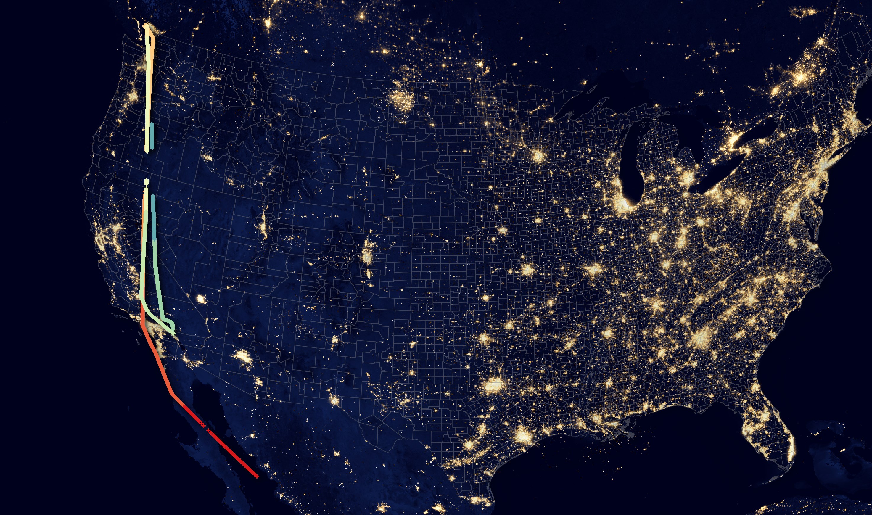
There are only 9 hours of data for this aircraft with a huge chunk between 5 AM and 5 PM missing.
SELECT   HOUR(trace.timestamp::TIMESTAMP) AS hour,
         COUNT(*)
FROM     READ_PARQUET('traces_*.pq')
WHERE    r = 'C-FSEQ'
GROUP BY 1
ORDER BY 1;
┌───────┬──────────────┐
│ hour  │ count_star() │
│ int64 │    int64     │
├───────┼──────────────┤
│     1 │          135 │
│     2 │          200 │
│     3 │          137 │
│     4 │          297 │
│    17 │          108 │
│    18 │          184 │
│    19 │          221 │
│    22 │          210 │
│    23 │          118 │
└───────┴──────────────┘
I looked up the Aircraft's movements on the 18th and 19th on FlightRadar24.
DATE        |   STD |   ATD |   STA | STATUS        | FLIGHT TIME | FLIGHT | FROM                  | TO
------------|-------|-------|-------|---------------|-------------|--------|-----------------------|-------------------
19 Nov 2023 | 23:10 | 00:16 | 06:59 | Delayed 07:30 |           — | AC536  | Kahului (OGG)         | Vancouver (YVR)
19 Nov 2023 | 17:25 | 18:35 | 21:57 | Landed 22:47  |        6:12 | AC537  | Vancouver (YVR)       | Kahului (OGG)
19 Nov 2023 | 13:10 | 14:04 | 16:14 | Landed 16:55  |        2:52 | AC1047 | Palm Springs (PSP)    | Vancouver (YVR)
19 Nov 2023 | 09:15 | 09:51 | 12:11 | Landed 12:05  |        2:15 | AC1046 | Vancouver (YVR)       | Palm Springs (PSP)
18 Nov 2023 | 17:45 | 18:02 | 21:00 | Landed 21:00  |        4:57 | AC971  | Puerto Vallarta (PVR) | Vancouver (YVR)
The times above are all local and the timestamps in the feed are UTC. The first record in ADSB.lol's dataset showed the aircraft over Mexico's Baja Peninsula heading north just after midnight but FlightRadar24 had this plane as sitting at Vancouver airport already.
It could be I picked a bad example to examine. I'll keep my eye on this project and fingers crossed its feeder community expands.
Generalising Routes
Below I'll walk through aggregating the location points into common routes. There is some quantising here as traces within 150 KM of one another will be merged together.
I'll first create a single Parquet file containing the timestamp for each point, its geometry, the registration number of the aircraft and the owner / operator.
$ ~/duckdb traces.duckdb
COPY (SELECT trace.timestamp AS timestamp,
             ST_ASTEXT(ST_POINT(trace.lon,
                                trace.lat)) geom,
             r,
             ownOp
      FROM READ_PARQUET('traces_*.pq')
) TO 'flights.2023.11.19.pq' (
    FORMAT 'PARQUET',
    CODEC  'ZSTD');
The following is a Python script that can be fed an airline's name as it appeared earlier in this post and a GeoPackage file of its generalised routes will be generated.
$ vi generalise_flows.py
from   datetime import timedelta

from   geopandas import GeoDataFrame
import movingpandas as mpd
import pandas as pd
from   shapely.wkt import loads
import typer


app = typer.Typer(rich_markup_mode='rich')


@app.command()
def main(source:str       = 'flights.2023.11.19.pq',
         airline:str      = 'DELTA AIR LINES INC',
         max_distance:int = 150_000,  # meters
         min_distance:int = 5_000,    # meters
         tolerance:int    = 100,      # MinDistanceGeneralizer
         min_stop_duration:int = 30): # minutes
    df = pd.read_parquet(source,
                         columns=['r',
                                  'geom',
                                  'timestamp'],
                         filters=[('ownOp', '=', airline)])

    df['geom']      = df['geom'].apply(lambda x: loads(x))
    df['timestamp'] = pd.to_datetime(df['timestamp'],
                                     format='mixed')

    traj_collection = \
        mpd.TrajectoryCollection(
                GeoDataFrame(df,
                             crs='4326',
                             geometry='geom'),
                'r',
                t='timestamp')

    trips = mpd.ObservationGapSplitter(traj_collection)\
               .split(gap=timedelta(minutes=30))

    generalized = mpd.MinDistanceGeneralizer(trips)\
                     .generalize(tolerance=tolerance)
    aggregator  = \
        mpd.TrajectoryCollectionAggregator(
                generalized,
                max_distance=max_distance,
                min_distance=min_distance,
                min_stop_duration=
                    timedelta(minutes=min_stop_duration))
    pts         = aggregator.get_significant_points_gdf()
    clusters    = aggregator.get_clusters_gdf()

    flows = aggregator.get_flows_gdf()
    flows.to_file('flows.%s.gpkg' % airline.lower()
                                           .replace(' ', '_'),
                  driver='GPKG',
                  layer='flows')


if __name__ == "__main__":
    app()
$ python generalise_flows.py --airline='WESTJET'
The above generated a 791-record, 217 KB GeoPackage file. There is a line string for each route along with a corresponding weight. Below are a few example records.
SELECT *
FROM ST_READ('flows.westjet.gpkg')
ORDER BY 1 DESC
LIMIT 10;
┌────────┬────────────────────────────────────────────────────────────────────────────────────────────┐
│ weight │                                            geom                                            │
│ int64  │                                          geometry                                          │
├────────┼────────────────────────────────────────────────────────────────────────────────────────────┤
│     42 │ LINESTRING (-123.3416303922652 49.018943629834254, -123.21162136000001 49.081320180000006) │
│     40 │ LINESTRING (-123.21162136000001 49.081320180000006, -123.3416303922652 49.018943629834254) │
│     36 │ LINESTRING (-113.00240801923077 49.72783672115384, -113.96255978461538 51.14109955384615)  │
│     30 │ LINESTRING (-115.52910320895522 50.31214205970149, -113.96255978461538 51.14109955384615)  │
│     29 │ LINESTRING (-111.55437918279569 51.15796140860215, -109.43430470454545 51.087078545454546) │
│     28 │ LINESTRING (-121.56794045454545 49.28060646464646, -119.93893659999999 49.80824688571429)  │
│     28 │ LINESTRING (-115.90751358823529 50.65116670588235, -115.52910320895522 50.31214205970149)  │
│     28 │ LINESTRING (-119.93893659999999 49.80824688571429, -121.56794045454545 49.28060646464646)  │
│     27 │ LINESTRING (-123.21162136000001 49.081320180000006, -121.56794045454545 49.28060646464646) │
│     27 │ LINESTRING (-117.55564436231884 50.08672591304348, -115.90751358823529 50.65116670588235)  │
├────────┴────────────────────────────────────────────────────────────────────────────────────────────┤
│ 10 rows                                                                                   2 columns │
└─────────────────────────────────────────────────────────────────────────────────────────────────────┘
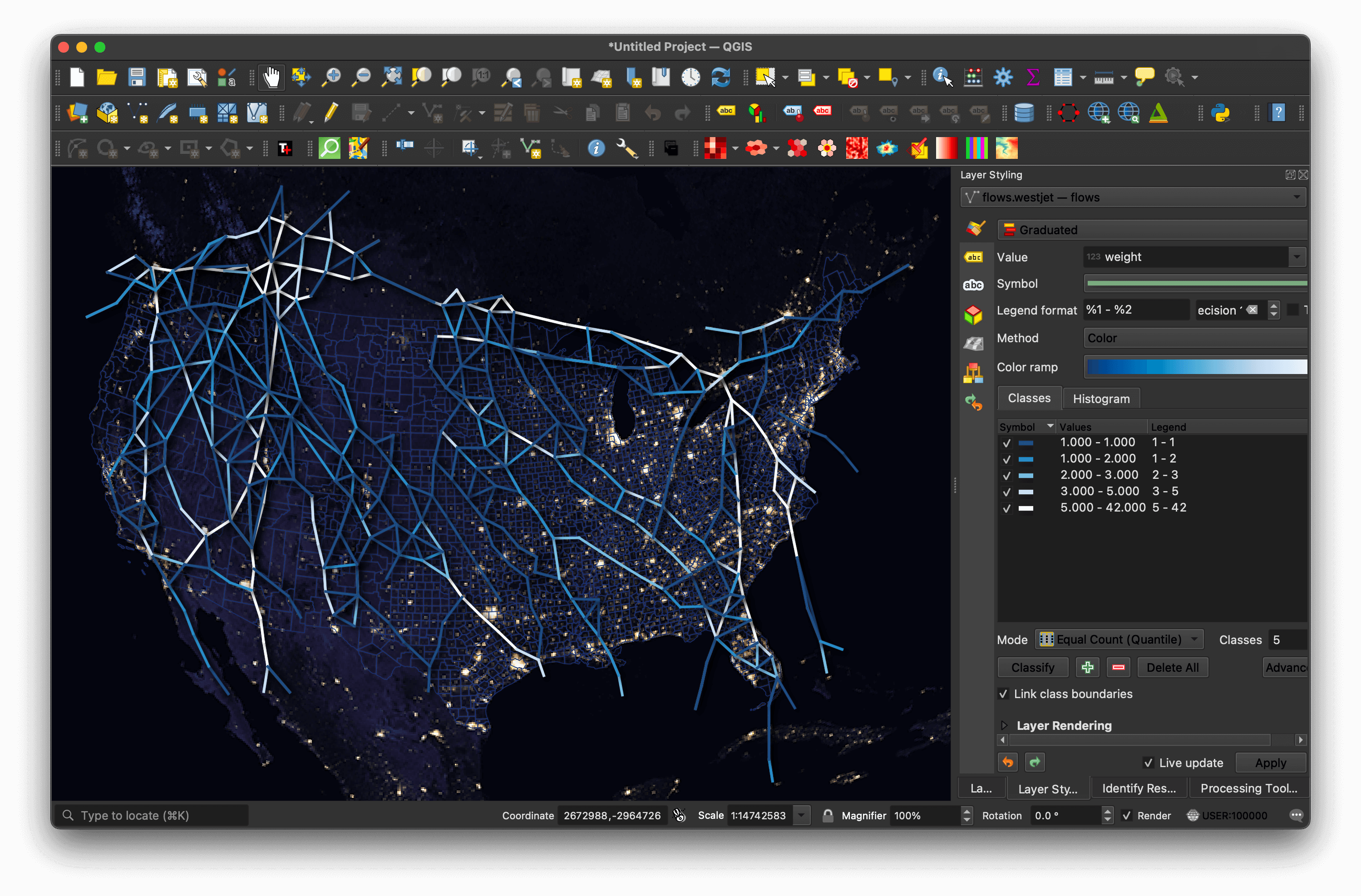
The following is a rendering of the above GeoPackage file in QGIS.
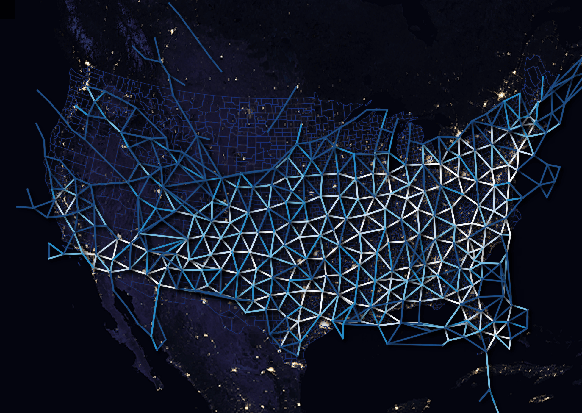
These are American Airlines' routes for the same day.
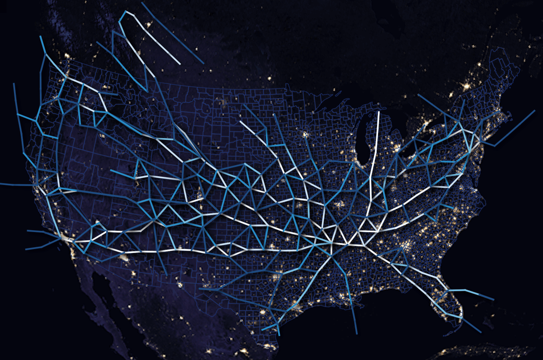
These are FedEx's routes.
It's fantastic that this data can be downloaded and examined with a simple laptop and relatively little friction.