Umbra Space is a 9-year-old manufacturer and operator of a Synthetic Aperture Radar (SAR) satellite fleet. These satellites can see through clouds, smoke and rain and can capture images day or night at resolutions as fine as 16cm. SpaceX launched Umbra's first satellite in 2021 and has a total of eight in orbit at the moment.
SAR collects images via radar waves rather than optically. The resolution of the resulting imagery can be improved the longer a point is captured as the satellite flies over the Earth. This also means video is possible as shown with this SAR imagery from another provider below.

Umbra has an open data programme where they share SAR imagery from 500+ locations around the world. The points on the map below are coloured based on the satellite that captured the imagery.
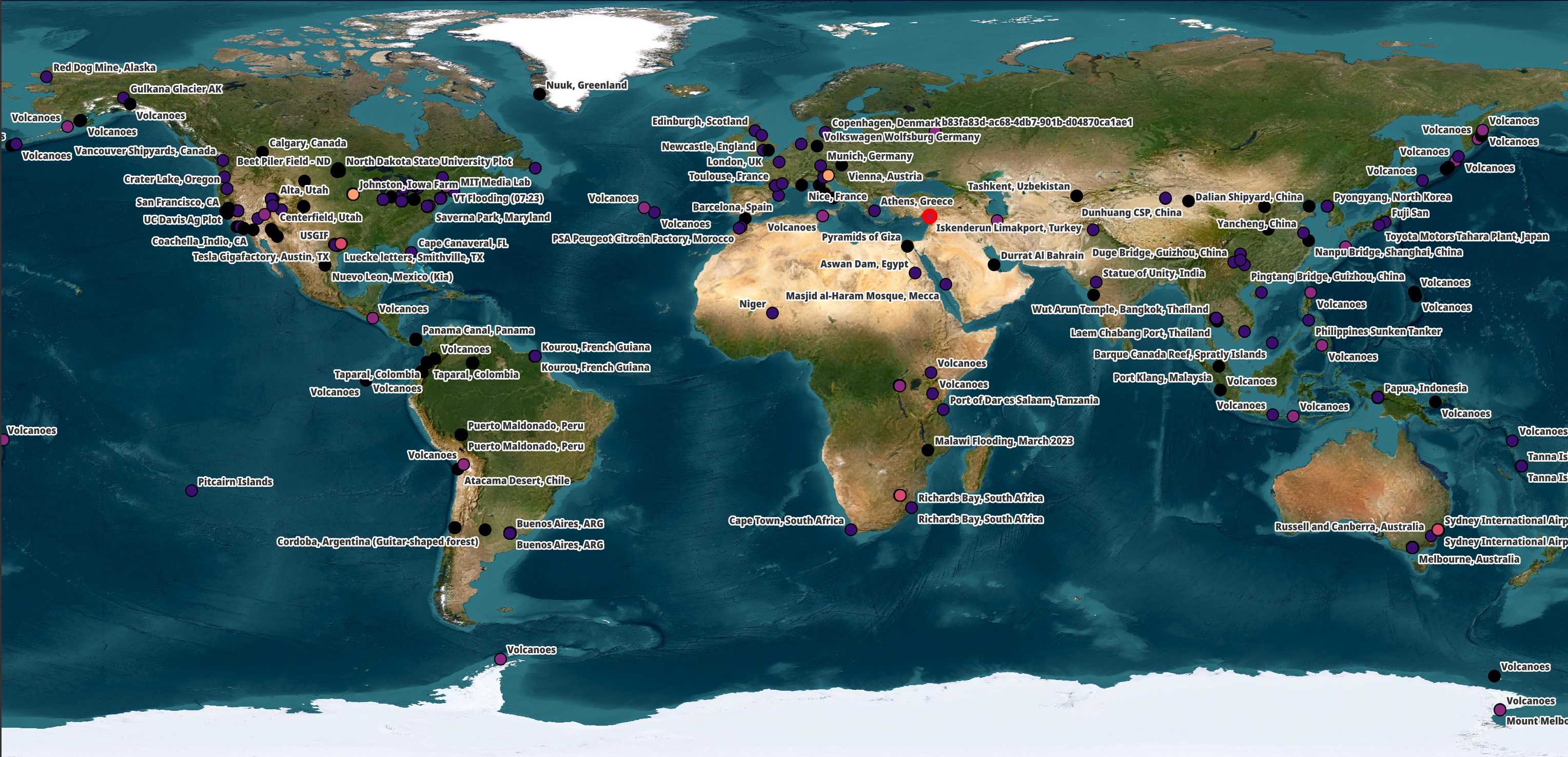
The subject matter largely focuses on manufacturing plants, airports, spaceports, large infrastructure projects and volcanos. Umbra state that the imagery being offered for free in their open data programme would have otherwise cost $4M to purchase.
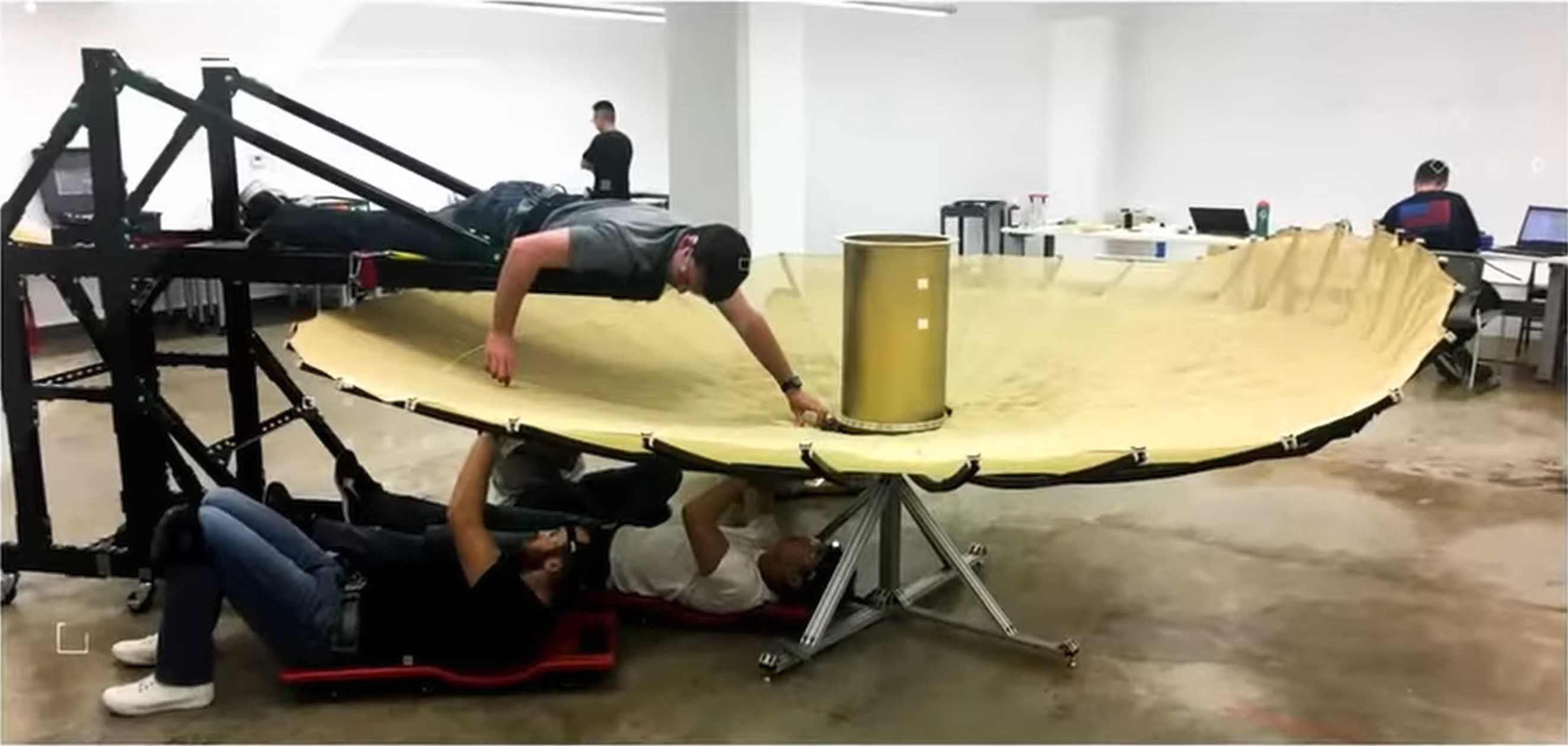
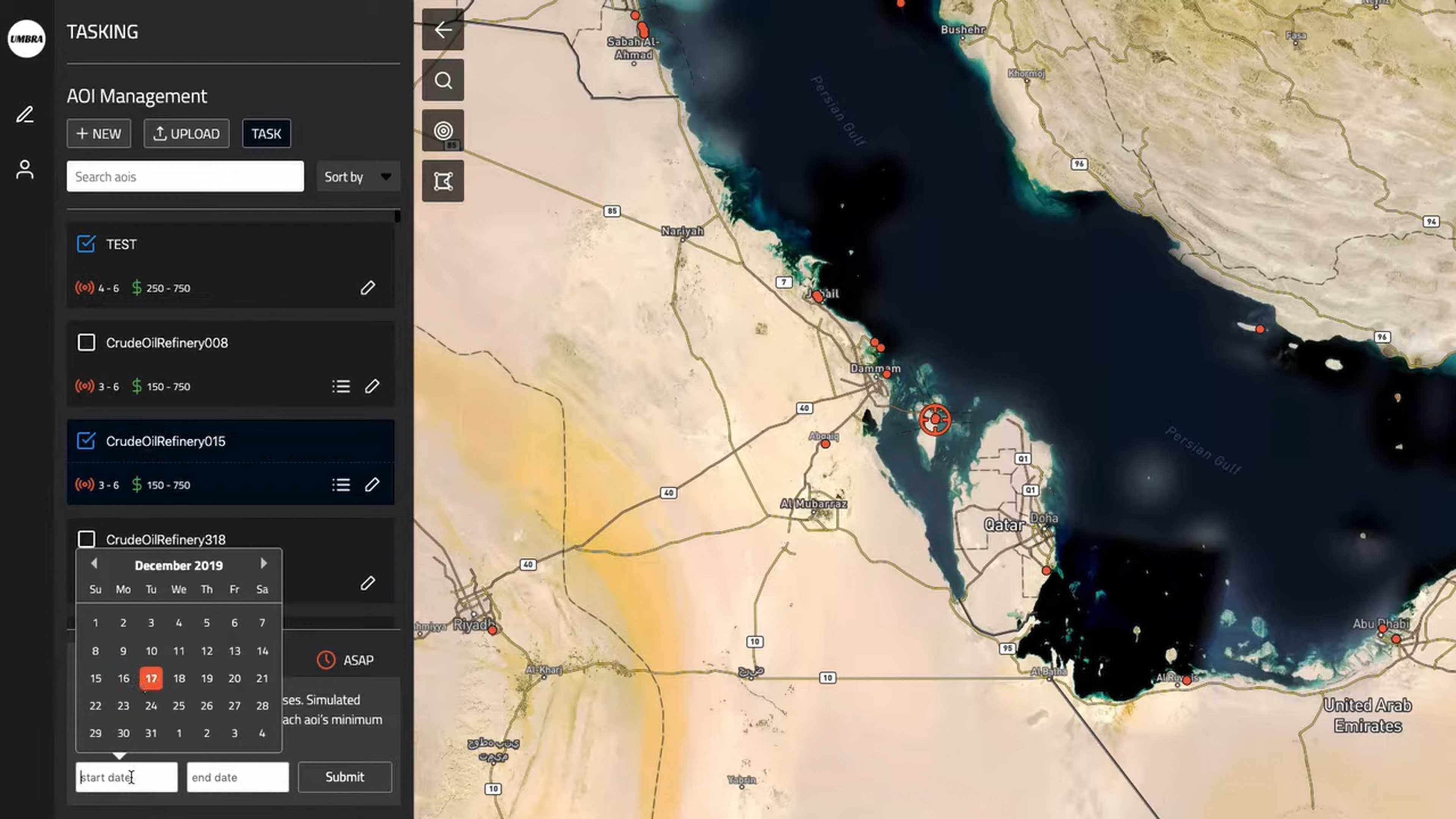
Below is a screenshot of Umbra's tasking UI. The company processes order as they arrived and don't allow customers to jump the queue.
In this post, I'll download and examine Umbra's freely available satellite imagery.
My Workstation
I'm using a 6 GHz Intel Core i9-14900K CPU. It has 8 performance cores and 16 efficiency cores with a total of 32 threads and 32 MB of L2 cache. It has a liquid cooler attached and is housed in a spacious, full-sized, Cooler Master HAF 700 computer case. I've come across videos on YouTube where people have managed to overclock the i9-14900KF to 9.1 GHz.
The system has 96 GB of DDR5 RAM clocked at 6,000 MT/s and a 5th-generation, Crucial T700 4 TB NVMe M.2 SSD which can read at speeds up to 12,400 MB/s. There is a heatsink on the SSD to help keep its temperature down. This is my system's C drive.
There is also an 8 TB HDD that will be used to store Umbra's Imagery.
The system is powered by a 1,200-watt, fully modular, Corsair Power Supply and is sat on an ASRock Z790 Pro RS Motherboard.
I'm running Ubuntu 22 LTS via Microsoft's Ubuntu for Windows on Windows 11 Pro. In case you're wondering why I don't run a Linux-based desktop as my primary work environment, I'm still using an Nvidia GTX 1080 GPU which has better driver support on Windows and I use ArcGIS Pro from time to time which only supports Windows natively.
Installing Prerequisites
I'll be using Python and a few other tools to help analyse the imagery in this post.
$ sudo apt update
$ sudo apt install \
    aws-cli \
    jq \
    libimage-exiftool-perl \
    libtiff-tools \
    libxml2-utils \
    python3-pip \
    python3-virtualenv \
    unzip
I'll set up a Python Virtual Environment and install a few packages.
$ virtualenv ~/.umbra
$ source ~/.umbra/bin/activate
$ python3 -m pip install \
    boto3 \
    rich \
    sarpy \
    shpyx
The sarpy package has a few issues with version 10 of Pillow so I'll downgrade it to the last version 9 that was released.
$ python3 -m pip install 'pillow<10'
I'll also use DuckDB, along with its JSON extension in this post.
$ cd ~
$ wget -c https://github.com/duckdb/duckdb/releases/download/v0.10.2/duckdb_cli-linux-amd64.zip
$ unzip -j duckdb_cli-linux-amd64.zip
$ chmod +x duckdb
$ ~/duckdb
INSTALL json;
I'll set up DuckDB to load every installed extension each time it launches.
$ vi ~/.duckdbrc
.timer on
.width 180
LOAD json;
Most of the maps in this post were rendered with QGIS version 3.36.1. QGIS is a desktop application that runs on Windows, macOS and Linux.
I used QGIS' Tile+ plugin to add Esri's World Imagery Basemap to each of the map renderings. This basemap helps provide visual context around Umbra's imagery.
I'll be using Google Earth's Desktop Application for some visualisations later on in the post.
Downloading Satellite Imagery
Umbra currently have 17 TB of files in their open data S3 bucket.
$ aws s3 ls --no-sign-request \
            --summarize \
            --human \
            --recursive \
            s3://umbra-open-data-catalog/ \
    | tail -n2
Total Objects: 20494
   Total Size: 17.1 TiB
Five types of files make up the majority of this bucket's contents. I'll download just the JSON and GeoTIFFs. These add up to ~1.3 TB in size.
$ for FORMAT in json tif; do
    aws s3 --no-sign-request \
           sync \
           --exclude="*" \
           --include="*.$FORMAT" \
           s3://umbra-open-data-catalog/ \
           ./
  done
I'll also download a single task's entire set of deliverables. These will be used to help explain the various formats Umbra delivers.
$ aws s3 --no-sign-request \
         sync \
         's3://umbra-open-data-catalog/sar-data/tasks/Beet Piler - ND' \
         ./sar-data/tasks
Umbra's Deliverables
Within any given task you can find one or more folders named with the starting time that the imagery was captured. This folder will usually include five different types of files. Below are some example file name and their respective file sizes.
589M ... 2023-11-19-16-12-16_UMBRA-05_CPHD.cphd
206M ... 2023-11-19-16-12-16_UMBRA-05_SICD.nitf
 49M ... 2023-11-19-16-12-16_UMBRA-05_GEC.tif
 39M ... 2023-11-19-16-12-16_UMBRA-05_SIDD.nitf
  4k ... 2023-11-19-16-12-16_UMBRA-05_METADATA.json
The naming convention is <date and time>_UMBRA-<satellite number>_<deliverable>.<file format>.
The first file format is Compensated Phase History Data (CPHD). These contain the lowest-level data and comes at an additional charge when ordering imagery. The files themselves can't be opened natively by QGIS or ArcGIS Pro. Below I'll extract the metadata from a CPHD file using sarpy.
$ python3
import json

from   sarpy.io.phase_history.converter import open_phase_history


reader = open_phase_history('2023-11-19-16-12-16_UMBRA-05_CPHD.cphd')
open('CPHD_metadata.json', 'w')\
    .write(json.dumps(reader.cphd_details.cphd_meta.to_dict(),
                      sort_keys=True,
                      indent=4))
The above produced a 770-line JSON file. Below are the top-level keys.
$ jq -S 'keys' CPHD_metadata.json
[
  "Antenna",
  "Channel",
  "CollectionID",
  "Data",
  "Dwell",
  "ErrorParameters",
  "Global",
  "PVP",
  "ProductInfo",
  "ReferenceGeometry",
  "SceneCoordinates",
  "SupportArray",
  "TxRcv"
]
Below is the reference geometry from this image.
$ jq -S '.ReferenceGeometry' CPHD_metadata.json
{
  "Monostatic": {
    "ARPPos": {
      "X": -248125.4300996695,
      "Y": -4820909.879421797,
      "Z": 4933637.577405307
    },
    "ARPVel": {
      "X": -2034.5657340855437,
      "Y": -5251.930139297333,
      "Z": -5207.0647911931055
    },
    "AzimuthAngle": 108.20119706650821,
    "DopplerConeAngle": 94.33891094952334,
    "GrazeAngle": 53.893258655900986,
    "GroundRange": 352505.5349499567,
    "IncidenceAngle": 36.106741344099014,
    "LayoverAngle": 99.82776516396562,
    "SideOfTrack": "R",
    "SlantRange": 649078.8128657481,
    "SlopeAngle": 54.18512696414206,
    "TwistAngle": 6.781795770580344
  },
  "ReferenceTime": 0.6976410888884236,
  "SRP": {
    "ECF": {
      "X": -552223.3276367188,
      "Y": -4332875,
      "Z": 4632556.640625
    },
    "IAC": {
      "X": 0,
      "Y": 0,
      "Z": 0
    }
  },
  "SRPCODTime": 0.6977821072510094,
  "SRPDwellTime": 1.3857412468969763
}
The second file format is Sensor Independent Complex Data (SCID). These files have SAR imagery that was processed through an image formation algorithm and are less idiosyncratic than CPHD. These files can be opened by both QGIS and ArcGIS Pro natively. Below I'll extract the metadata from an SCID file using sarpy.
$ python3
import json

from   sarpy.io.complex.converter import open_complex


reader = open_complex('2023-11-19-16-12-16_UMBRA-05_SICD.nitf')
open('SICD_metadata.json', 'w')\
    .write(json.dumps(reader.get_sicds_as_tuple()[0].to_dict(),
                      sort_keys=True,
                      indent=4))
The above produced 1,466 lines of JSON. Below are the top-level keys.
$ jq -S 'keys' SICD_metadata.json
[
  "Antenna",
  "CollectionInfo",
  "ErrorStatistics",
  "GeoData",
  "Grid",
  "ImageCreation",
  "ImageData",
  "ImageFormation",
  "PFA",
  "Position",
  "RadarCollection",
  "Radiometric",
  "SCPCOA",
  "Timeline"
]
These are the satellite's locations as it took 32 captures that produced the final image.
$ jq -c '.GeoData.ValidData[]' SICD_metadata.json
{"Lat":46.85362559857068,"Lon":-97.24599513287323,"index":1}
{"Lat":46.85497237569043,"Lon":-97.2522503236929,"index":2}
{"Lat":46.856318810715116,"Lon":-97.25850582747549,"index":3}
{"Lat":46.85766490359525,"Lon":-97.26476164409529,"index":4}
{"Lat":46.85901065428136,"Lon":-97.27101777342662,"index":5}
{"Lat":46.86035606272401,"Lon":-97.27727421534378,"index":6}
{"Lat":46.861701128873726,"Lon":-97.28353096972094,"index":7}
{"Lat":46.86304585268113,"Lon":-97.28978803643231,"index":8}
{"Lat":46.86439023409682,"Lon":-97.296045415352,"index":9}
{"Lat":46.86868214345577,"Lon":-97.29408543110029,"index":10}
{"Lat":46.872974016177125,"Lon":-97.29212513429353,"index":11}
{"Lat":46.87726585219771,"Lon":-97.29016452486162,"index":12}
{"Lat":46.8815576514544,"Lon":-97.28820360273428,"index":13}
{"Lat":46.88584941388401,"Lon":-97.28624236784137,"index":14}
{"Lat":46.89014113942342,"Lon":-97.2842808201126,"index":15}
{"Lat":46.89443282800942,"Lon":-97.28231895947772,"index":16}
{"Lat":46.8987244795789,"Lon":-97.28035678586649,"index":17}
{"Lat":46.89737924912188,"Lon":-97.27409580578416,"index":18}
{"Lat":46.89603367590721,"Lon":-97.26783513866391,"index":19}
{"Lat":46.89468775998437,"Lon":-97.26157478463178,"index":20}
{"Lat":46.89334150140286,"Lon":-97.25531474381373,"index":21}
{"Lat":46.89199490021218,"Lon":-97.2490550163357,"index":22}
{"Lat":46.89064795646192,"Lon":-97.24279560232362,"index":23}
{"Lat":46.889300670201585,"Lon":-97.23653650190332,"index":24}
{"Lat":46.88795304148079,"Lon":-97.2302777152006,"index":25}
{"Lat":46.88366224066232,"Lon":-97.23224348871302,"index":26}
{"Lat":46.87937140270454,"Lon":-97.23420894885537,"index":27}
{"Lat":46.87508052767064,"Lon":-97.2361740956979,"index":28}
{"Lat":46.8707896156238,"Lon":-97.23813892931099,"index":29}
{"Lat":46.86649866662721,"Lon":-97.2401034497648,"index":30}
{"Lat":46.86220768074405,"Lon":-97.24206765712964,"index":31}
{"Lat":46.85791665803749,"Lon":-97.24403155147571,"index":32}
Below are the processing steps this image went through.
$ jq -S '.ImageFormation.Processings' ICD_metadata.json
[
  {
    "Applied": true,
    "Parameters": {
      "kazimuth": "fixed",
      "krange": "fixed"
    },
    "Type": "inscription"
  },
  {
    "Applied": true,
    "Type": "Valkyrie Systems Sage | Umbra CPHD processor 0.7.5.1 @ 2023-11-20T03:03:03.474347Z"
  },
  {
    "Applied": true,
    "Parameters": {
      "PulseRFIDataFractionRemoved:Primary": "0.00039429605910101806",
      "PulseRFIPowerFractionRemoved:Primary": "7.450580596923828e-06"
    },
    "Type": "Valkyrie Systems Sage | CPHD Pulse RFI Removal 0.4.8.0 @ 2023-11-20T03:03:07.211039Z"
  },
  {
    "Applied": true,
    "Parameters": {
      "constant_type": "two_dimensional",
      "linear_type": "two_dimensional",
      "phase_contiguous": "true",
      "quadratic_type": "two_dimensional"
    },
    "Type": "polar_deterministic_phase"
  }
]
The third file format is Sensor Independent Derived Data (SIDD). This file includes coordinate and product image pixel array data. These files can be opened by both QGIS and ArcGIS Pro natively.
$ python3
import json

from   sarpy.io.product.converter import open_product


reader = open_product('2023-11-19-16-12-16_UMBRA-05_SIDD.nitf')

open('SIDD_metadata.json', 'w')\
    .write(json.dumps(reader.get_sidds_as_tuple()[0].to_dict(),
                      sort_keys=True,
                      indent=4))
The above produced 652 lines of JSON.
$ jq -S 'keys' SIDD_metadata.json
[
  "Display",
  "ErrorStatistics",
  "ExploitationFeatures",
  "GeoData",
  "Measurement",
  "ProductCreation",
  "ProductProcessing"
]
Below is a rich amount of imagery collection details.
$ jq -S '.ExploitationFeatures.Collections' SIDD_metadata.json
[
  {
    "Geometry": {
      "Azimuth": 108.20086921413612,
      "DopplerConeAngle": 94.3387327601436,
      "Graze": 53.89328163094832,
      "Slope": 54.18512623664181,
      "Squint": -97.78483972720454,
      "Tilt": 6.78152241416755
    },
    "Information": {
      "CollectionDateTime": "2023-11-19T16:12:17.000000Z",
      "CollectionDuration": 1.3928192466125595,
      "RadarMode": {
        "ModeType": "SPOTLIGHT"
      },
      "Resolution": {
        "Azimuth": 0.9955238668720371,
        "Range": 0.5906637804745409
      },
      "SensorName": "Umbra-05"
    },
    "Phenomenology": {
      "GroundTrack": 97.24478337121614,
      "Layover": {
        "Angle": -172.4134911153026,
        "Magnitude": 1.3857758071085169
      },
      "MultiPath": -175.29876491419682,
      "Shadow": {
        "Angle": -0.7865835230301172,
        "Magnitude": 0.7293921722527886
      }
    },
    "identifier": "2023-11-19T16:12:17_Umbra-05"
  }
]
The fourth file format, Geo-Ellipsoid Corrected Data (GEC), is a GeoTIFF file. These files can be opened by both QGIS and ArcGIS Pro natively. I'll cover them more later on in this post.
The fifth file is a JSON-formatted metadata file. These contain a large amount of information about where and how the image was captured. Below are the top-level keys.
$ jq -S . 2023-06-24-06-55-55_UMBRA-06_METADATA.json \
    | jq 'del(.derivedProducts)' \
    | jq 'del(.collects)'
{
  "baseIpr": 0.35,
  "imagingMode": "SPOTLIGHT",
  "orderType": "SNAPSHOT",
  "productSku": "UMB-SPOTLIGHT-35-1",
  "targetIpr": 0.35,
  "umbraSatelliteName": "UMBRA_06",
  "vendor": "Umbra Space",
  "version": "1.0.0"
}
The capture start and end times are also recorded. The following shows this image was captured over ~4.2 seconds.
$ jq -S '[.collects[0].startAtUTC,.collects[0].endAtUTC]' \
    2023-06-24-06-55-55_UMBRA-06_METADATA.json
[
  "2023-06-24T06:55:56.949411+00:00",
  "2023-06-24T06:56:01.151960+00:00"
]
GeoJSON of the image's footprint can be extracted from the JSON metadata file.
$ jq -S '.collects[0].footprintPolygonLla' \
    2023-11-19-16-12-16_UMBRA-05_METADATA.json \
    > footprint.geojson
There is also a large amount of detail describing the capture process.
$ jq -S '.collects[0]' 2023-06-24-06-55-55_UMBRA-06_METADATA.json \
    | jq -S 'del(.footprintPolygonLla)'
{
  "angleAzimuthDegrees": -24.578109794554347,
  "angleGrazingDegrees": 51.0925454012932,
  "angleIncidenceDegrees": 38.9074545987068,
  "angleSquintDegrees": 129.99928283691406,
  "antennaGainDb": 0,
  "endAtUTC": "2023-06-24T06:56:01.151960+00:00",
  "id": "497b9cd9-a0d9-496e-b80d-0b85a7be50b0",
  "maxGroundResolution": {
    "azimuthMeters": 0.356073504716498,
    "rangeMeters": 0.35362660311636107
  },
  "observationDirection": "LEFT",
  "polarizations": [
    "VV"
  ],
  "radarBand": "X",
  "radarCenterFrequencyHz": 9600001353.88691,
  "revisitId": null,
  "satelliteTrack": "DESCENDING",
  "sceneCenterPointLla": {
    "coordinates": [
      -114.06925107327962,
      51.04910910790581,
      1057.6477352934555
    ],
    "type": "Point"
  },
  "slantRangeMeters": 670809.7686782589,
  "startAtUTC": "2023-06-24T06:55:56.949411+00:00",
  "taskId": "82fc4627-cfac-46c6-a889-d6df4418e360",
  "timeOfCenterOfAperturePolynomial": {
    "Coefs": [
      [
        2.611847181373054
      ]
    ]
  }
}
I'll collect all of the JSON metadata files' contents into a single JSONL file and examine it in DuckDB.
$ python3
from   glob import glob
import json


with open('footprints.json', 'w') as f:
    for filename in glob('sar-data/tasks/*/*/*.json') + \
                    glob('sar-data/tasks/*/*/*/*.json'):
        f.write(json.dumps(json.loads(open(filename, 'r').read())) + '\n')
$ ~/duckdb
Below are the ground resolution buckets for all of the imagery across this dataset.
SELECT ROUND(LIST_EXTRACT(collects, 1).maxGroundResolution.azimuthMeters, 1) azimuthMeters,
       COUNT(*)
FROM READ_JSON('footprints.json')
GROUP BY 1
ORDER BY 1;
┌───────────────┬──────────────┐
│ azimuthMeters │ count_star() │
│    double     │    int64     │
├───────────────┼──────────────┤
│           0.1 │            1 │
│           0.2 │          155 │
│           0.3 │          408 │
│           0.4 │          426 │
│           0.5 │          623 │
│           0.6 │          211 │
│           0.7 │           20 │
│           0.8 │          114 │
│           0.9 │          144 │
│           1.0 │          134 │
│           1.1 │           52 │
│           1.2 │           57 │
│           1.3 │            9 │
│           1.4 │           17 │
│           1.5 │           24 │
│           1.6 │           15 │
│           1.7 │            9 │
│           1.8 │            2 │
│           2.0 │            1 │
├───────────────┴──────────────┤
│ 19 rows            2 columns │
└──────────────────────────────┘
SELECT ROUND(LIST_EXTRACT(collects, 1).maxGroundResolution.rangeMeters, 1) rangeMeters,
       COUNT(*)
FROM READ_JSON('footprints.json')
GROUP BY 1
ORDER BY 1;
┌─────────────┬──────────────┐
│ rangeMeters │ count_star() │
│   double    │    int64     │
├─────────────┼──────────────┤
│         0.2 │           44 │
│         0.3 │          340 │
│         0.4 │          503 │
│         0.5 │          654 │
│         0.6 │          169 │
│         0.7 │           18 │
│         0.8 │          148 │
│         0.9 │          168 │
│         1.0 │          201 │
│         1.1 │           58 │
│         1.2 │           42 │
│         1.3 │           11 │
│         1.4 │           24 │
│         1.5 │           18 │
│         1.6 │           15 │
│         1.7 │            6 │
│         1.8 │            1 │
│         1.9 │            2 │
├─────────────┴──────────────┤
│ 18 rows          2 columns │
└────────────────────────────┘
Geo-Ellipsoid Corrected Data
The GEC files Umbra delivers are Cloud-Optimised GeoTIFF containers. These files contain Tiled Multi-Resolution TIFFs / Tiled Pyramid TIFFs. This means there are several versions of the same image at different resolutions within the TIFF file.
These files are structured so it's easy to only read a portion of a file for any one resolution you're interested in. A file might be 100 MB but a JavaScript-based Web Application might only need to download 2 MB of data from that file in order to render its lowest resolution.
Below I'll write a parser to convert the output from tiffinfo into JSON for each GEC file and include its corresponding satellite metadata.
$ python3
import json
from   pathlib       import Path
import re
from   shlex         import quote
import sys

from   rich.progress import track
from   shpyx         import run as execute


def parse_tiff(lines:list):
    stack, stack_id = {}, None

    for line in lines:
        if not stack_id:
            stack_id = 1
        elif line.startswith('TIFF Directory'):
            stack_id = stack_id + 1
        elif line.startswith('  ') and line.count(':') == 1:
            if stack_id not in stack.keys():
                stack[stack_id] = {'stack_num': stack_id}

            x, y = line.strip().split(':')

            if len(x) > 1 and not x.startswith('Tag ') and \
               y and \
               len(str(y).strip()) > 1:
                stack[stack_id][x.strip()] = y.strip()
        elif line.startswith('  ') and \
             line.count(':') == 2 and \
             'Image Width' in line:
            if stack_id not in stack.keys():
                stack[stack_id] = {'stack_num': stack_id}

            _, width, _, _, _ = re.split(r'\: ([0-9]*)', line)
            stack[stack_id]['width'] = int(width.strip())

    return [y for x, y in stack.items()]


with open('umbra_metadata.jsonl', 'w') as f:
    for path in track(list(Path('sar-data/tasks').rglob('*.tif'))):
        lines = execute('tiffinfo -i %s' % quote(path.absolute().as_posix()))\
                    .stdout\
                    .strip()\
                    .splitlines()

        try:
            sat_meta = json.loads(open(list(Path(path.parent)
                                                .rglob('*.json'))[0], 'r')
                                    .read())
        except:
            sat_meta = {}

        for line in parse_tiff(lines):
            f.write(json.dumps({**line,
                                **{'filename': path.absolute().as_posix(),
                                   'sat_meta': sat_meta}},
                               sort_keys=True) + '\n')
I'll load the JSON into a DuckDB table.
$ ~/duckdb
CREATE OR REPLACE TABLE umbra AS
    SELECT * FROM
    READ_JSON('umbra_metadata.jsonl');
Umbra's GEC files can contain up to 9 images / stacks. The larger stack files are produced by the entire fleet and aren't limited to just a few of Umbra's satellites.
SELECT  stack_num,
         COUNT(*) FILTER (WHERE sat_meta.umbraSatelliteName = 'UMBRA_04') AS UMBRA_04,
         COUNT(*) FILTER (WHERE sat_meta.umbraSatelliteName = 'UMBRA_05') AS UMBRA_05,
         COUNT(*) FILTER (WHERE sat_meta.umbraSatelliteName = 'UMBRA_06') AS UMBRA_06,
         COUNT(*) FILTER (WHERE sat_meta.umbraSatelliteName = 'UMBRA_07') AS UMBRA_07,
         COUNT(*) FILTER (WHERE sat_meta.umbraSatelliteName = 'UMBRA_08') AS UMBRA_08
FROM     umbra
GROUP BY 1
ORDER BY 1;
┌───────────┬──────────┬──────────┬──────────┬──────────┬──────────┐
│ stack_num │ UMBRA_04 │ UMBRA_05 │ UMBRA_06 │ UMBRA_07 │ UMBRA_08 │
│   int64   │  int64   │  int64   │  int64   │  int64   │  int64   │
├───────────┼──────────┼──────────┼──────────┼──────────┼──────────┤
│         1 │     1314 │     1528 │      618 │      186 │       68 │
│         2 │     1198 │     1329 │      482 │      118 │       38 │
│         3 │     1198 │     1328 │      482 │      118 │       38 │
│         4 │     1198 │     1328 │      482 │      118 │       38 │
│         5 │     1130 │     1253 │      464 │      118 │       38 │
│         6 │      807 │      878 │      336 │       90 │       27 │
│         7 │      268 │      249 │      123 │       26 │       11 │
│         8 │       47 │       41 │       19 │        0 │        1 │
│         9 │        1 │        0 │        0 │        0 │        0 │
└───────────┴──────────┴──────────┴──────────┴──────────┴──────────┘
There does seem to be a pattern where the wider and taller deliverables tend to have a larger stack but this isn't always the case.
SELECT   round(list_extract(sat_meta.derivedProducts.GEC, 1).numColumns / 10000) * 10000 as cols,
         COUNT(*) FILTER (WHERE stack_num = 1) AS stack_num_1,
         COUNT(*) FILTER (WHERE stack_num = 2) AS stack_num_2,
         COUNT(*) FILTER (WHERE stack_num = 3) AS stack_num_3,
         COUNT(*) FILTER (WHERE stack_num = 4) AS stack_num_4,
         COUNT(*) FILTER (WHERE stack_num = 5) AS stack_num_5,
         COUNT(*) FILTER (WHERE stack_num = 6) AS stack_num_6,
         COUNT(*) FILTER (WHERE stack_num = 7) AS stack_num_7,
         COUNT(*) FILTER (WHERE stack_num = 8) AS stack_num_8,
         COUNT(*) FILTER (WHERE stack_num = 9) AS stack_num_9
FROM     umbra
GROUP BY 1
ORDER BY 1;
┌─────────┬─────────────┬─────────────┬─────────────┬─────────────┬─────────────┬─────────────┬─────────────┬─────────────┬─────────────┐
│  cols   │ stack_num_1 │ stack_num_2 │ stack_num_3 │ stack_num_4 │ stack_num_5 │ stack_num_6 │ stack_num_7 │ stack_num_8 │ stack_num_9 │
│ double  │    int64    │    int64    │    int64    │    int64    │    int64    │    int64    │    int64    │    int64    │    int64    │
├─────────┼─────────────┼─────────────┼─────────────┼─────────────┼─────────────┼─────────────┼─────────────┼─────────────┼─────────────┤
│     0.0 │         307 │         307 │         307 │         307 │         146 │           0 │           0 │           0 │           0 │
│ 10000.0 │        2069 │        1909 │        1909 │        1909 │        1909 │        1190 │           2 │           0 │           0 │
│ 20000.0 │        1150 │         791 │         790 │         790 │         790 │         790 │         519 │          33 │           0 │
│ 30000.0 │         179 │         150 │         150 │         150 │         150 │         150 │         148 │          67 │           0 │
│ 40000.0 │           6 │           6 │           6 │           6 │           6 │           6 │           6 │           6 │           0 │
│ 50000.0 │           2 │           1 │           1 │           1 │           1 │           1 │           1 │           1 │           0 │
│ 60000.0 │           1 │           1 │           1 │           1 │           1 │           1 │           1 │           1 │           1 │
└─────────┴─────────────┴─────────────┴─────────────┴─────────────┴─────────────┴─────────────┴─────────────┴─────────────┴─────────────┘
Only around 1/7th of the imagery is LZW-compressed. More lossless compression use could have a big impact on the current ~1.3 TB disk footprint and bandwidth requirements needed to download the GEC files off of S3.
SELECT   "Compression Scheme",
         COUNT(*) FILTER (WHERE sat_meta.umbraSatelliteName = 'UMBRA_04') AS UMBRA_04,
         COUNT(*) FILTER (WHERE sat_meta.umbraSatelliteName = 'UMBRA_05') AS UMBRA_05,
         COUNT(*) FILTER (WHERE sat_meta.umbraSatelliteName = 'UMBRA_06') AS UMBRA_06,
         COUNT(*) FILTER (WHERE sat_meta.umbraSatelliteName = 'UMBRA_07') AS UMBRA_07,
         COUNT(*) FILTER (WHERE sat_meta.umbraSatelliteName = 'UMBRA_08') AS UMBRA_08
FROM     umbra
GROUP BY 1
ORDER BY 1;
┌────────────────────┬──────────┬──────────┬──────────┬──────────┬──────────┐
│ Compression Scheme │ UMBRA_04 │ UMBRA_05 │ UMBRA_06 │ UMBRA_07 │ UMBRA_08 │
│      varchar       │  int64   │  int64   │  int64   │  int64   │  int64   │
├────────────────────┼──────────┼──────────┼──────────┼──────────┼──────────┤
│ LZW                │      914 │     1467 │      981 │      505 │      220 │
│ None               │     6247 │     6466 │     2025 │      269 │       39 │
└────────────────────┴──────────┴──────────┴──────────┴──────────┴──────────┘
Colour Sub-Aperture Imagery
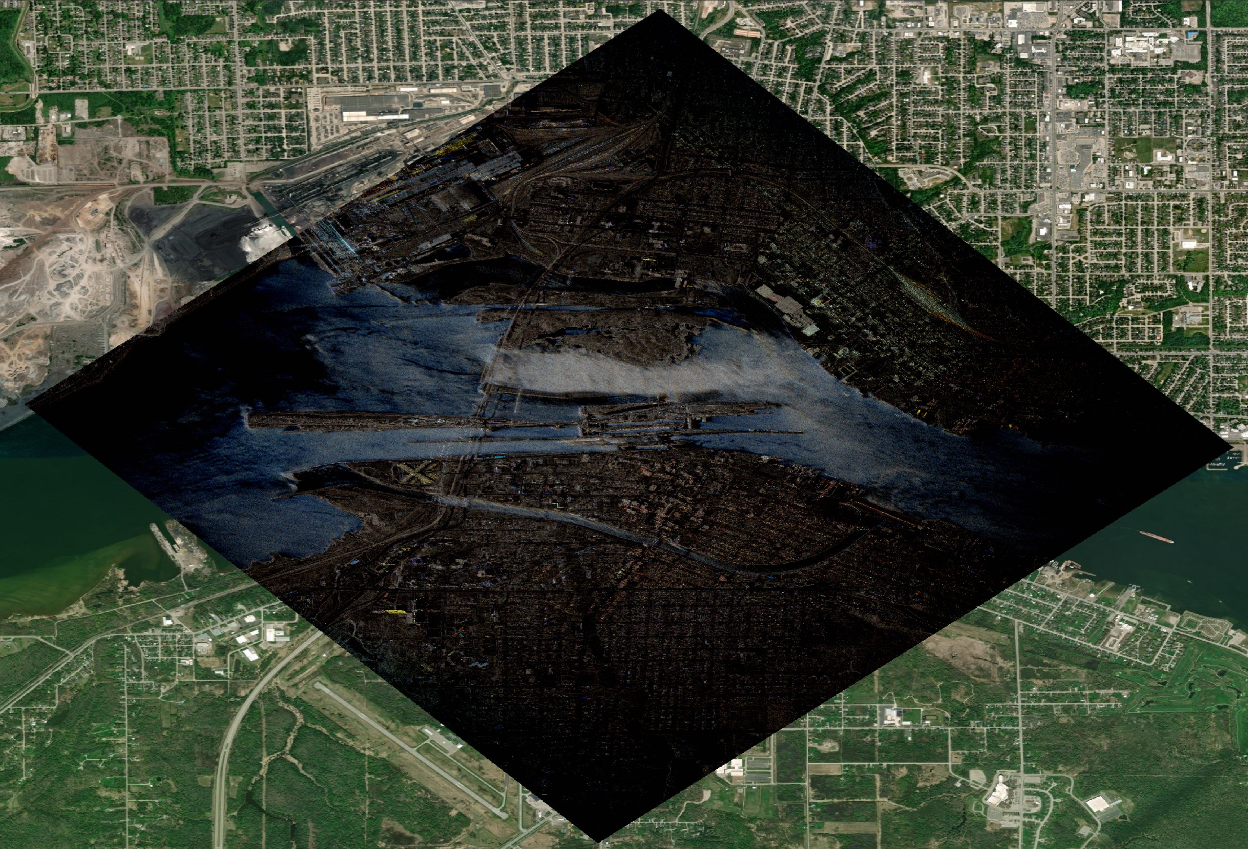
After my initial publication of this blog, I found out Umbra also delivers Colour Sub-Aperture Imagery (CSI). Todd Master, Umbra's COO, stated on LinkedIn that CSI can help identify man-made or moving objects more easily.
Below is one of their recent examples taken in Michigan.
$ wget http://umbra-open-data-catalog.s3.amazonaws.com/sar-data/tasks/ad%20hoc/SooLocks_MI/de5bd5e2-acf2-4669-826b-9e028dfc193f/2024-05-15-02-50-45_UMBRA-04/2024-05-15-02-50-45_UMBRA-04_CSI.tif
I suspect this is done using a false-colour technique Scott Manley described in his SAR explained video. Below I can see colour interpretation metadata in this file which I haven't seen in Umbra's other deliverables.
$ exiftool '2024-05-15-02-50-45_UMBRA-04_CSI.tif' \
    | grep COLORINTERP \
    | grep -o '<GDAL.*' \
    | sed 's/>./>/g' \
    | xmllint --format -
<?xml version="1.0"?>
<GDALMetadata>
  <Item name="COLLECT_ID">618ddf4-ca85-44b6-9120-be1f6726dd12</Item>
  <Item name="PROCESSOR">.43.0</Item>
  <Item name="COLORINTERP" sample="0" role="colorinterp">ndefined</Item>
  <Item name="COLORINTERP" sample="1" role="colorinterp">ndefined</Item>
  <Item name="COLORINTERP" sample="2" role="colorinterp">ndefined</Item>
</GDALMetadata>
As of May 21st, 2024, I found 830 CSI deliverables from 118 locations.
$ aws s3 --no-sign-request \
       ls \
       --recursive \
       s3://umbra-open-data-catalog/ \
    | grep CSI.tif \
    > CSIs.txt

$ (grep -v 'ad hoc' CSIs.txt | cut -d'/' -f3;
   grep 'ad hoc' CSIs.txt | cut -d'/' -f4) \
    | sort \
    | uniq \
    | wc -l
118
I've noticed these files tend to be twice the size of their GEC counterparts and can often be over 1 GB each.
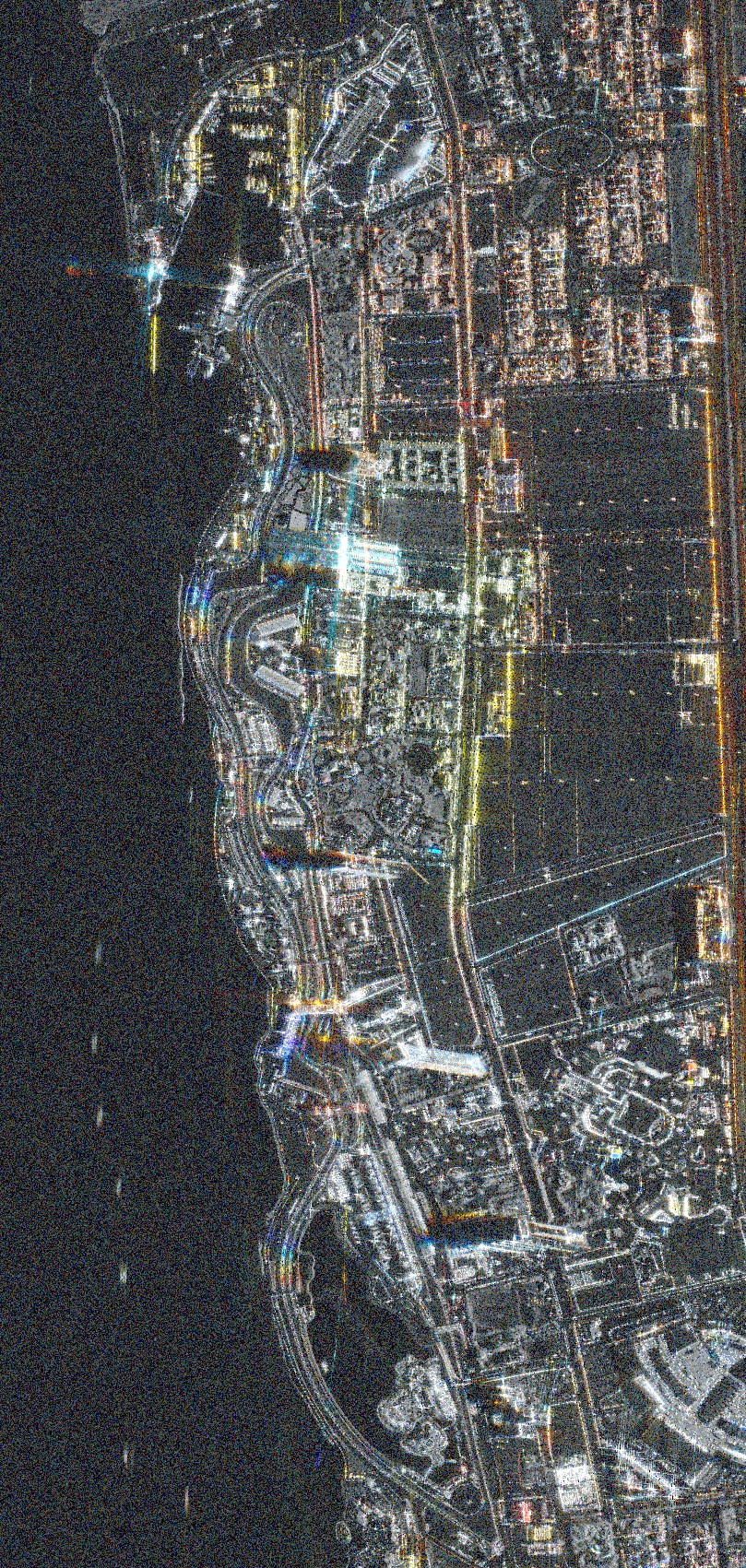
Below is the Formula 1 Street Circuit in Saudi Arabia.
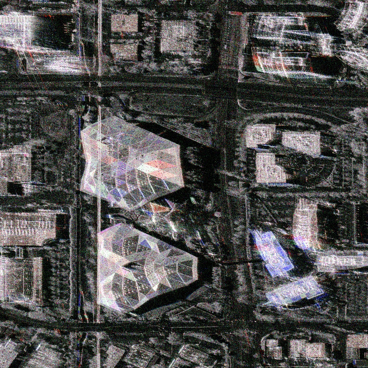
Nvidia's Headquarters in Santa Clara look very colourful and stand out well.
Umbra on Google Earth
The SICD files Umbra deliver can be ~7x larger than GEC files. But when spot-checking, I found they can be 4,000 pixels taller (13018 x 17264 for SICD versus 13218 x 13219 for GEC). There is a utility in sarpy that converts SICD files into Google Earth's KMZ files.
Converting to KMZ took ~25 seconds for each SICD file on my Intel Core i9-14900K. The resulting KMZ files are 50x smaller and often only a few MB in size. They can be loaded almost immediately in Google Earth.
Below I'll fetch the URIs of the imagery of BMW's car plants around the world.
$ python3
from   shlex           import quote

import boto3
from   botocore        import UNSIGNED
from   botocore.config import Config


def get_all_s3_objects(s3, **base_kwargs):
    continuation_token = None

    while True:
        list_kwargs = dict(MaxKeys=1000, **base_kwargs)

        if continuation_token:
            list_kwargs['ContinuationToken'] = continuation_token

        response = s3.list_objects_v2(**list_kwargs)
        yield from response.get('Contents', [])

        if not response.get('IsTruncated'):
            break

        continuation_token = response.get('NextContinuationToken')


s3_client = boto3.client('s3', config=Config(signature_version=UNSIGNED))
bmw_files = []

for s3_file in get_all_s3_objects(
                    s3_client,
                    Bucket='umbra-open-data-catalog',
                    Prefix='sar-data/tasks/ad hoc/25-cm resolution images/'):
    if 'bmw'  in s3_file['Key'].lower() and \
       'SICD' in s3_file['Key'].upper():
        bmw_files.append(s3_file)

bash_cmd = 'aws s3 cp --no-sign-request ' \
           '"s3://umbra-open-data-catalog/%s" %s\n'

with open('bmw.sh', 'w') as f:
    for uri in bmw_files:
        city_name = uri['Key'].split('/')[5]\
                              .replace(', ', '_')\
                              .replace(' ', '_')\
                              .lower()
        f.write(bash_cmd % (uri['Key'],
                            quote('./bmw_%s_SICD.nitf' % city_name)))
The above found ~26 GB of data across 14 SICD files. I'll run the following to download and convert them into KMZ.
$ bash -x bmw.sh

$ for FILENAME in bmw_*_SICD.nitf; do
    echo $FILENAME
    python3 -m sarpy.utils.create_kmz $FILENAME ./
  done
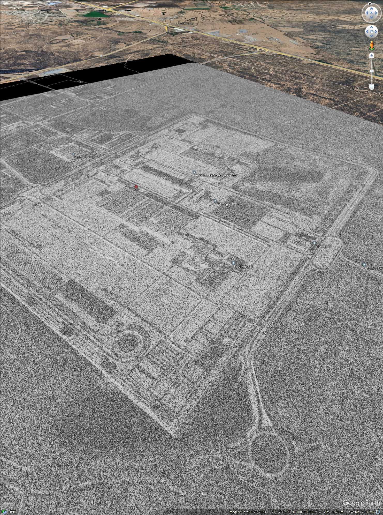
This is BMW's Factory in Mexico. Neither the Mexico nor Chinese plant locations have any 3D buildings in Google Earth so the SAR imagery renders well out of the box.
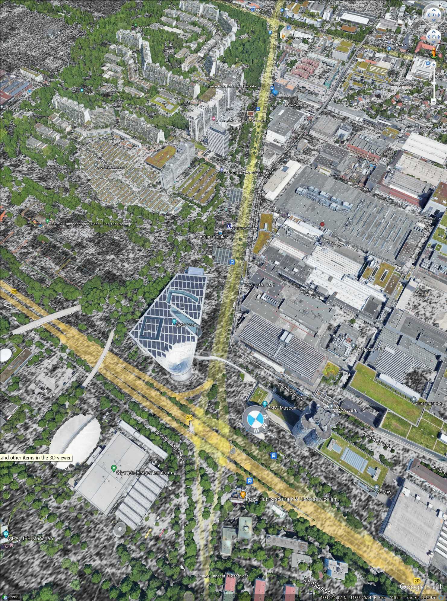
Google Earth doesn't displace the SAR imagery over its 3D buildings like ArcGIS Pro does so the factories in Germany, Austria, the UK, South Africa and South Carolina all look strange when the 3D buildings layer is enabled.
Imagery of Interest
The clarity of Umbra's SAR Imagery of McMurdo Station in Antarctica is second only to Google Maps' Satellite Imagery. Below is Umbra's SAR image on a displaced terrain model.
Many of the GEC files I looked at didn't line up well with other imagery. I'm not sure if this is a characteristic of how SAR is captured but it doesn't seem to be strictly related to the unique positions the satellites would have captured their respective imagery from.
I played around with georeferencing for a while but I couldn't find a common theme or offset that made sense. It was like stretching silly puddy to get an entire GEC image to align with any other Imagery provider I have access to.
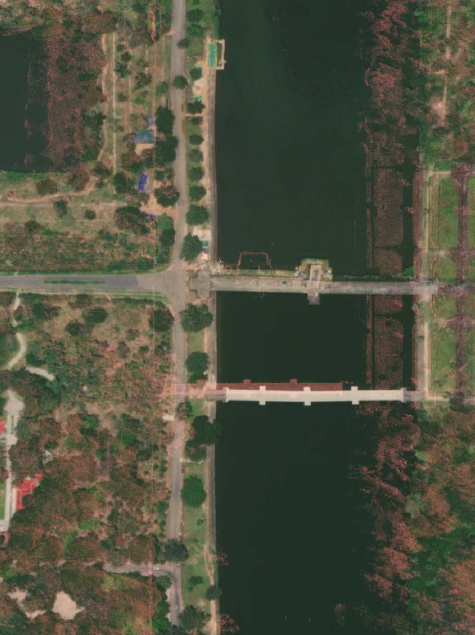
Below is a bridge in Angkor Wat, Cambodia. I've coloured Umbra's SAR image red. The bridge appears to sit 50 meters west and ~2.5 meters north of Esri's image of the same location.
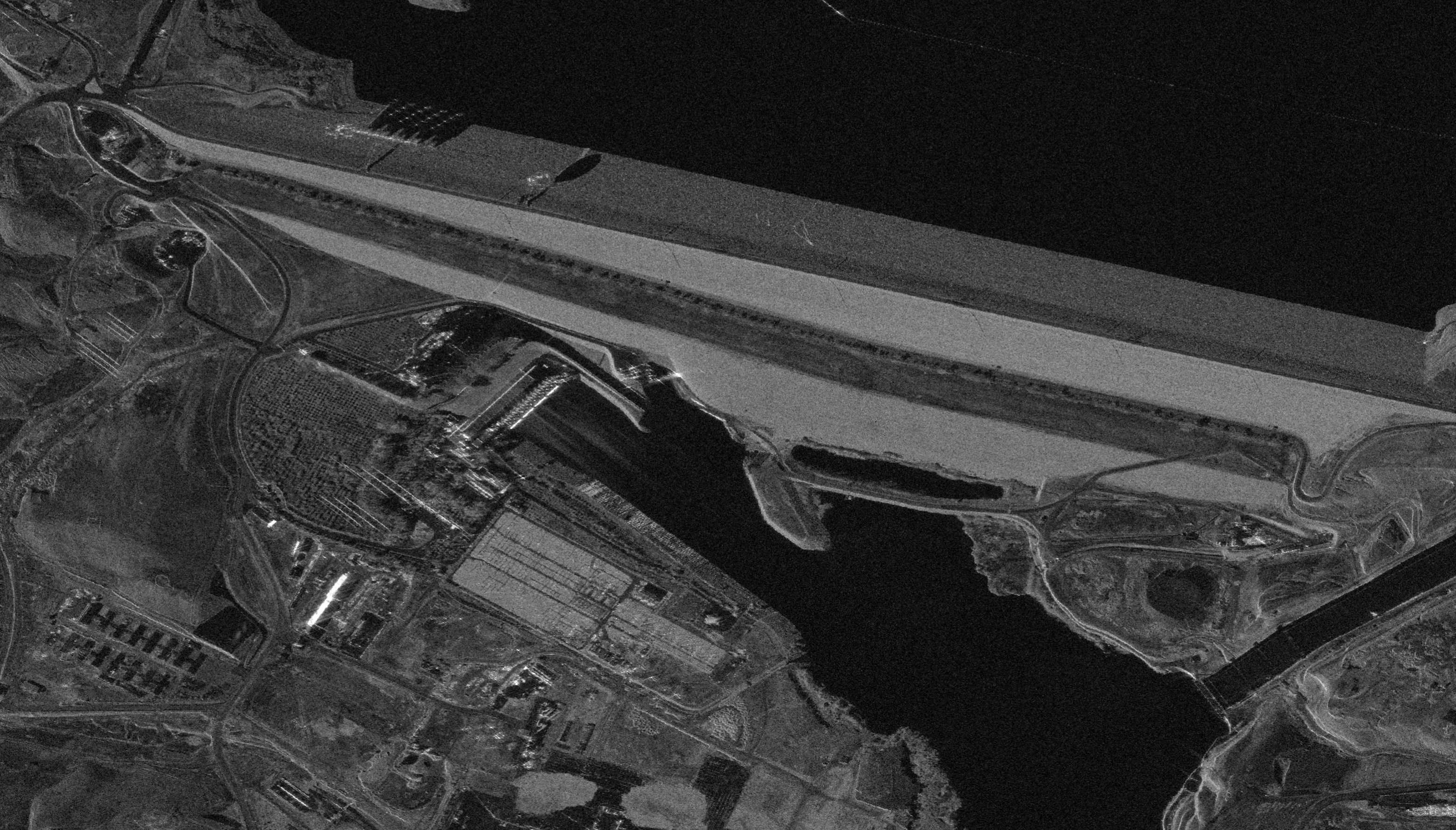
SAR Imagery is unique in that it can see at night and through clouds but I've noticed it can't pick up signage that would be otherwise visible in RGB imagery. Below is Esri's image of the Mosul Dam in Iraq. There is a massive sign with the Dam's name written in English on it.
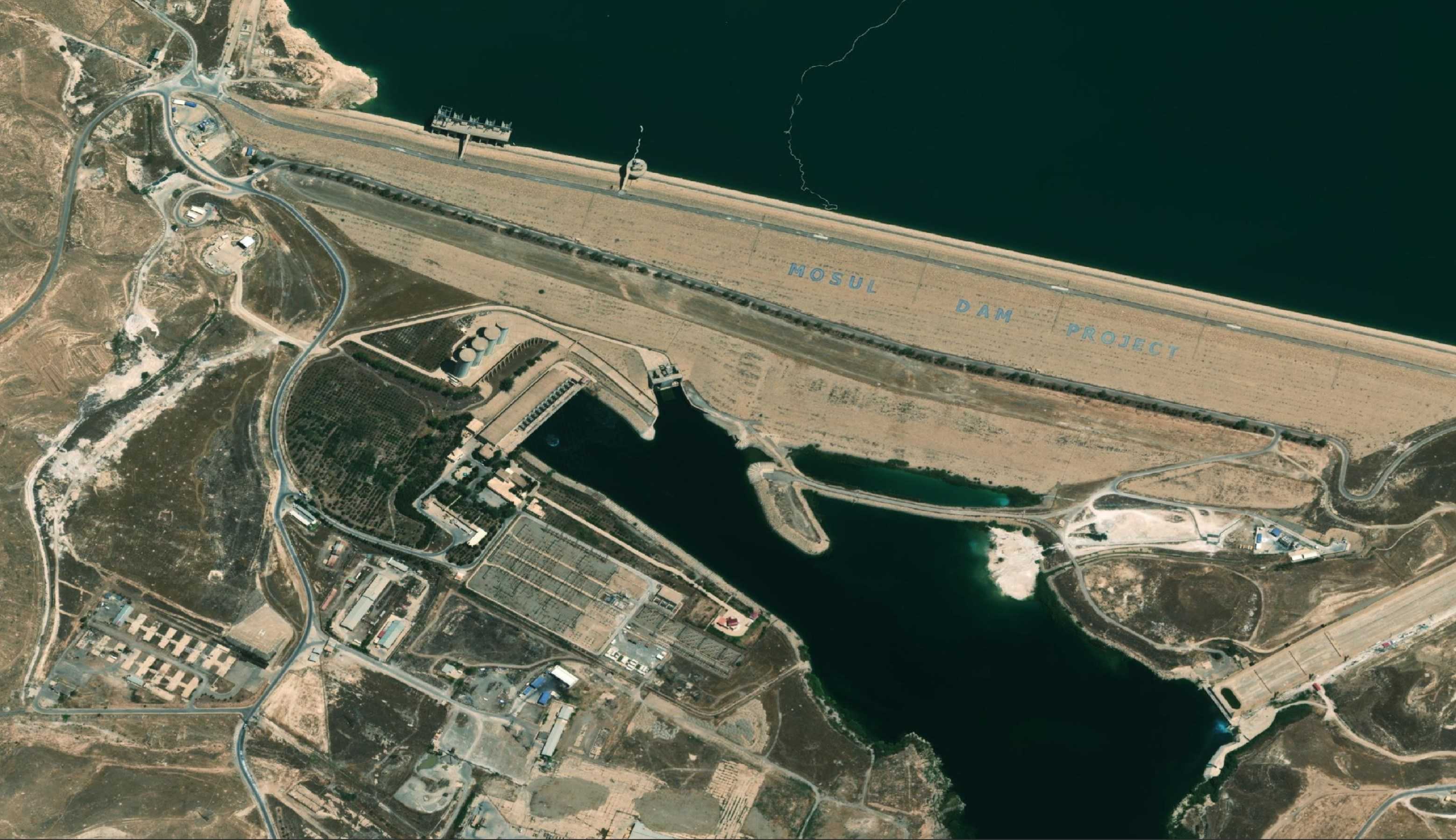
This sign isn't visible in Umbra's imagery. I suspect this is a limitation of SAR.
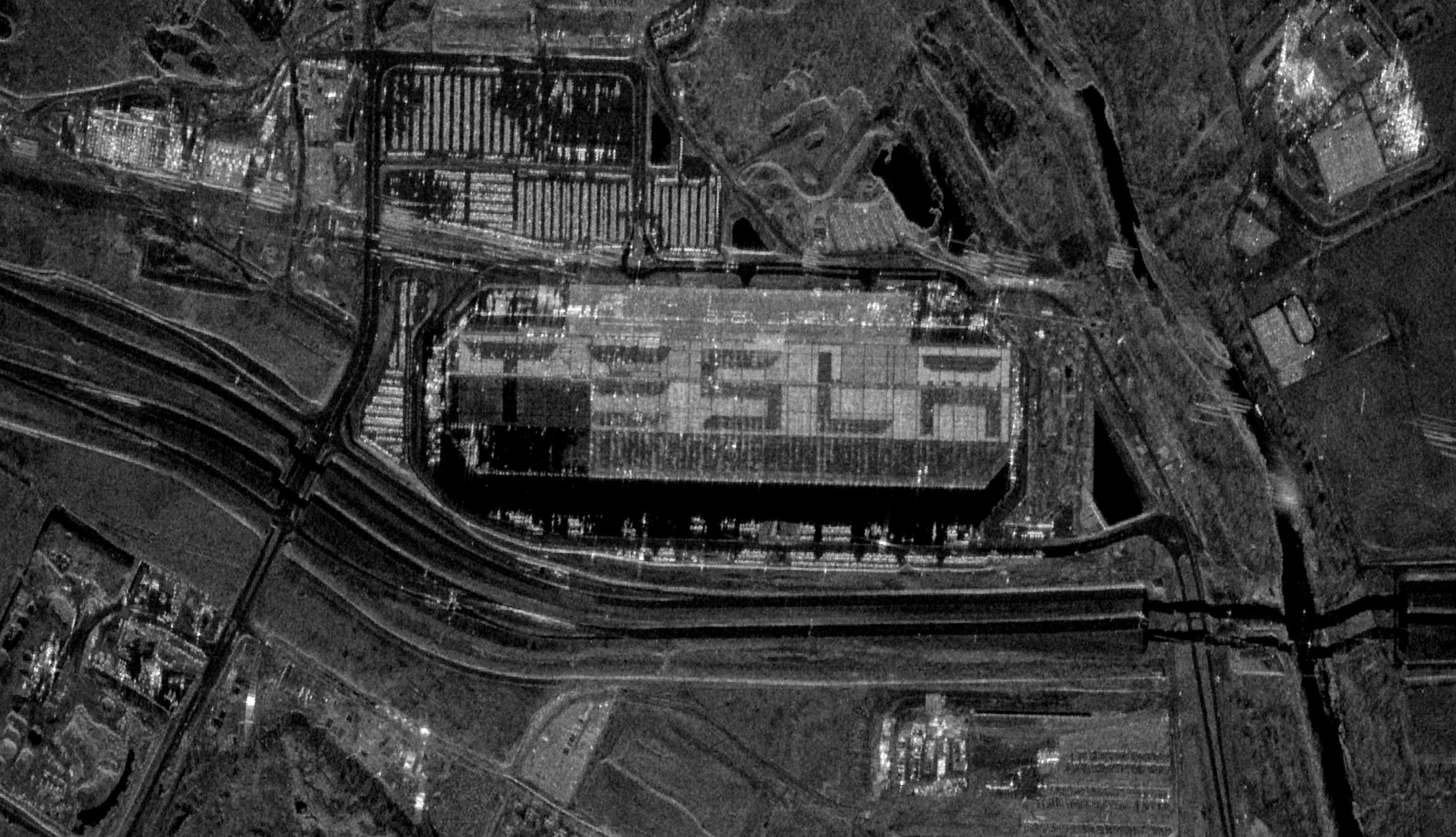
That said, Elon made sure this wouldn't be a problem when he built his Gigafactory in Austin, Texas.
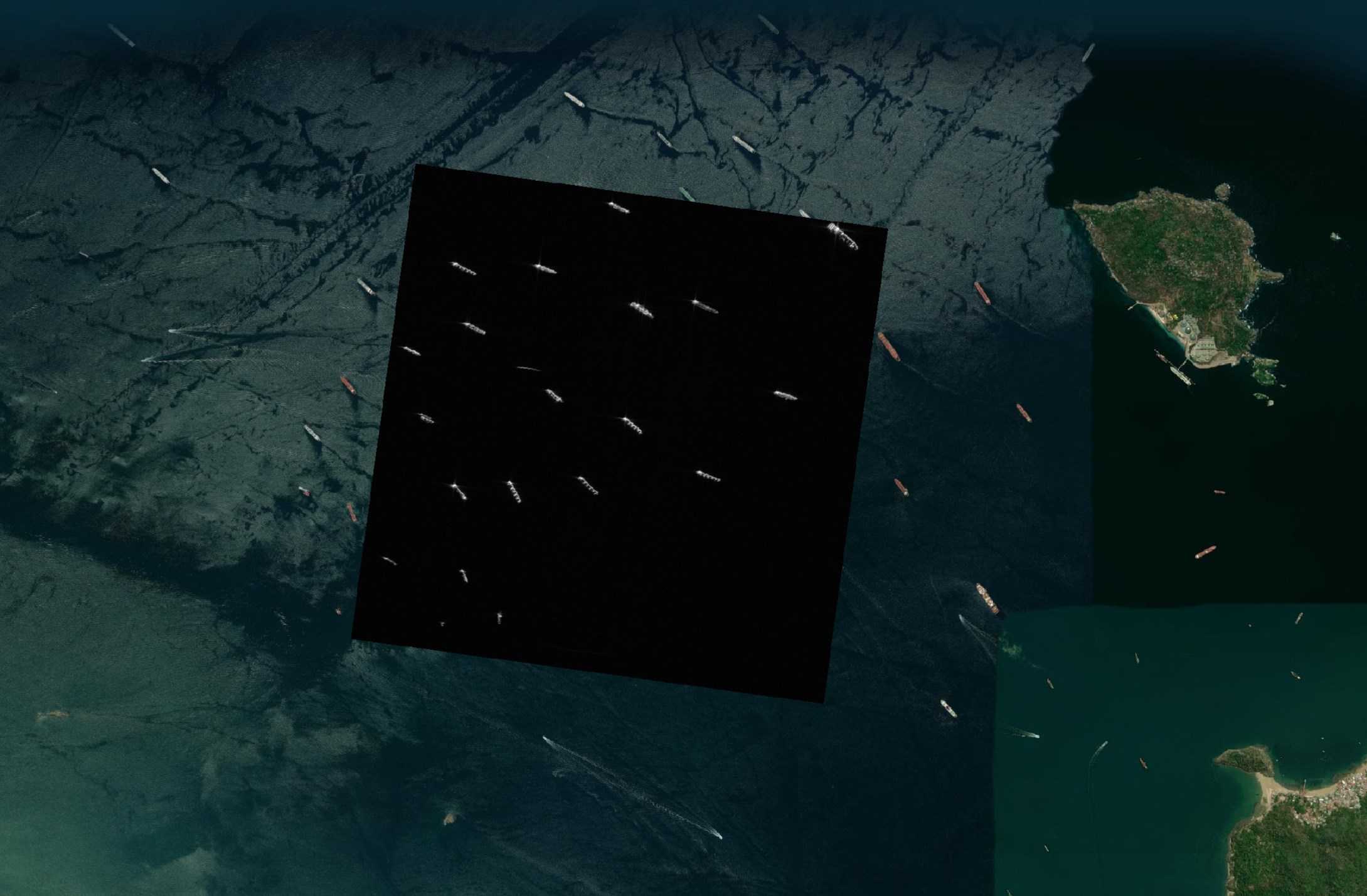
Boats contrast extremely well in SAR Imagery. This is an image Umbra took in Panama.
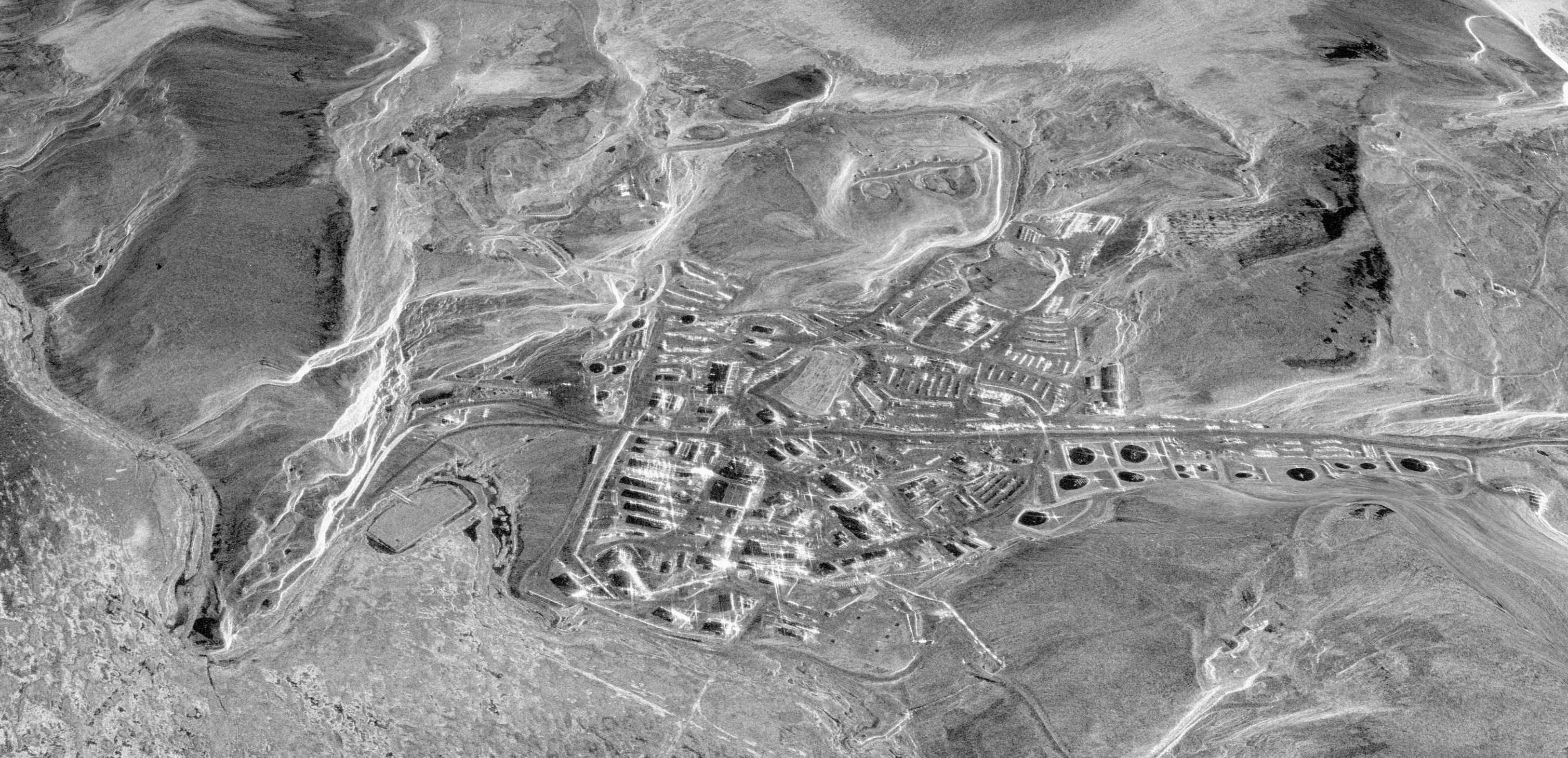
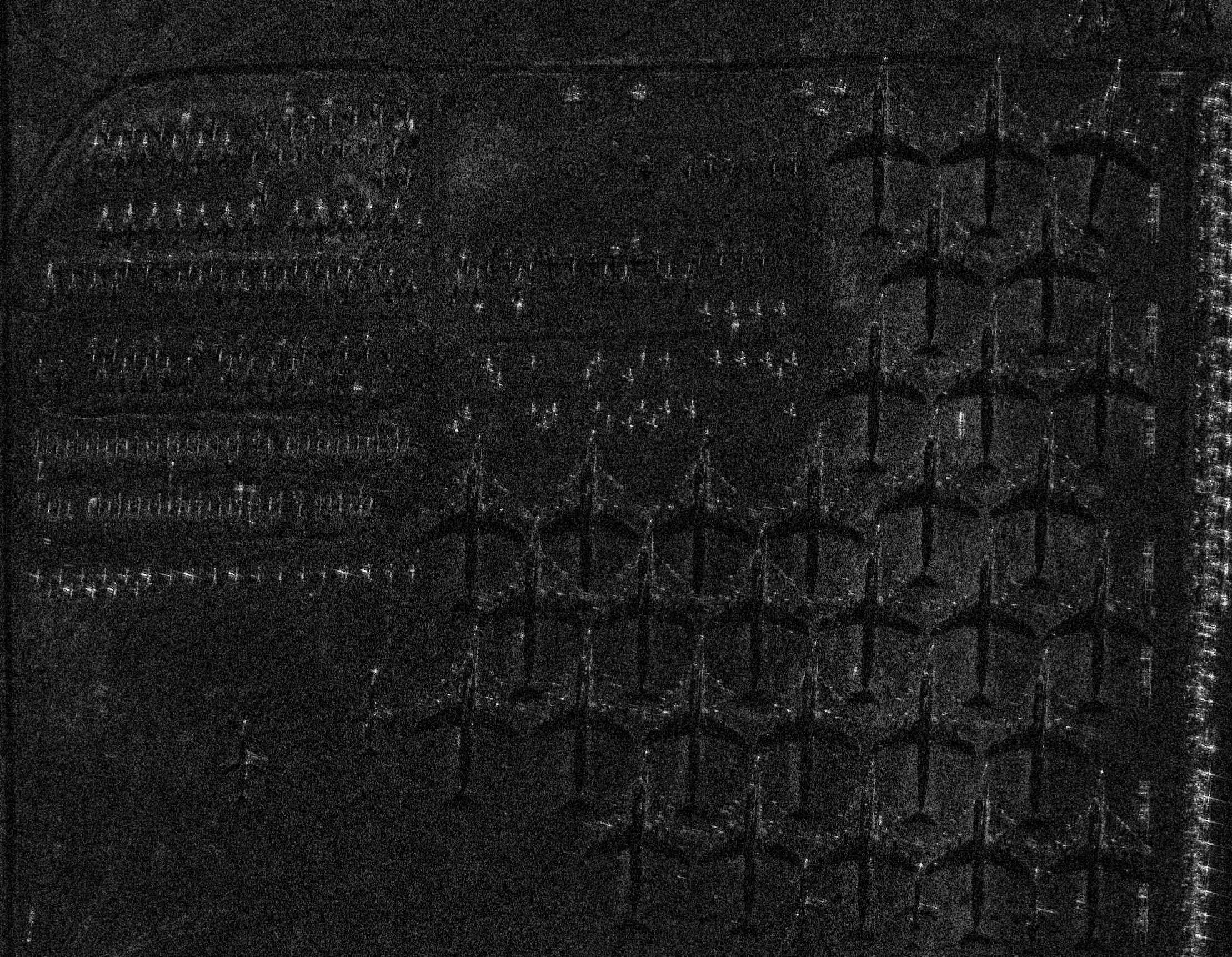
SAR can have blindspots. It can see things millimetres in size but objects between 10s of centimetres and a few meters can be invisible to SAR. The following is Esri's image of an aircraft boneyard. Though taken on different days, across every satellite imagery provider I have access to there were roughly the same number of planes parked at this location.
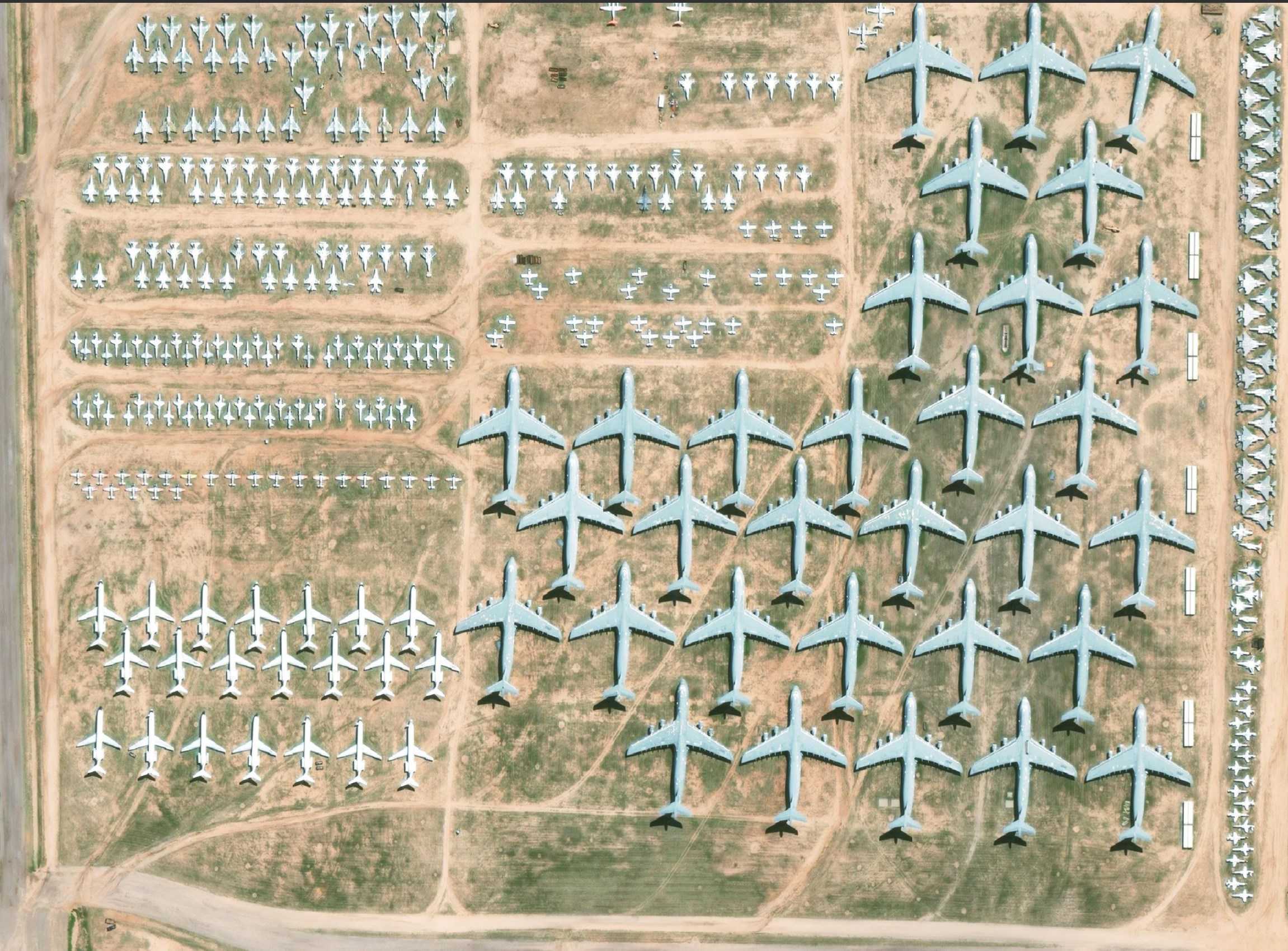
A lot of those planes aren't visible in Umbra's SAR image.
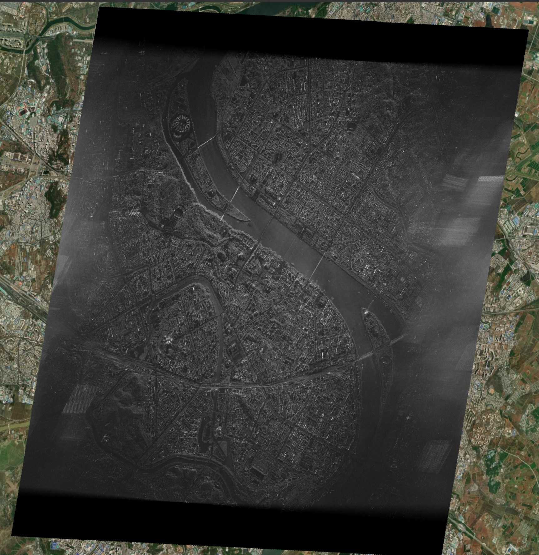
Nearly every image in Umbra's dataset is free of any major distortions but I found their 25cm-resolution image of Kim Il Sung Square in Pyongyang, North Korea had a lot of vignetting around the edges. This was taken with their fourth satellite.