Satellogic is a satellite designer, manufacturer and constellation operator. They were founded in 2010 and have offices in Argentina, Uruguay, Spain and the US.
They launched three prototype Cube satellites between 2013 and 2014, using China and Russia as their launch partners.
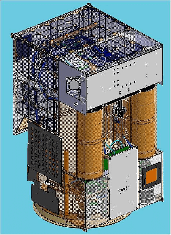
In 2016, they began launching ~38 KG, 10K-component, 51 x 57 x 82-cm NewSat microsatellites. These take around three months to build and are meant to last for three years in orbit. They've named the constellation of these satellites "Aleph-1".
Below is a rendering of their NewSat satellite.
They're aiming to have 300 satellites in orbit at some point which would provide revisit times up to every 5 minutes.
Last week, Satellogic announced an open satellite feed programme and named their dataset "Satellogic EarthView".
In this post, I'll examine Satellogic's constellation and open data feed.
My Workstation
I'm using a 6 GHz Intel Core i9-14900K CPU. It has 8 performance cores and 16 efficiency cores with a total of 32 threads and 32 MB of L2 cache. It has a liquid cooler attached and is housed in a spacious, full-sized Cooler Master HAF 700 computer case. I've come across videos on YouTube where people have managed to overclock the i9-14900KF to 9.1 GHz.
The system has 96 GB of DDR5 RAM clocked at 6,000 MT/s and a 5th-generation, Crucial T700 4 TB NVMe M.2 SSD which can read at speeds up to 12,400 MB/s. There is a heatsink on the SSD to help keep its temperature down. This is my system's C drive.
The system is powered by a 1,200-watt, fully modular Corsair Power Supply and is sat on an ASRock Z790 Pro RS Motherboard.
I'm running Ubuntu 22 LTS via Microsoft's Ubuntu for Windows on Windows 11 Pro. In case you're wondering why I don't run a Linux-based desktop as my primary work environment, I'm still using an Nvidia GTX 1080 GPU which has better driver support on Windows and I use ArcGIS Pro from time to time which only supports Windows natively.
Installing Prerequisites
I'll use GDAL 3.4.1, Python 3.8 and a few other tools to help analyse the data in this post.
$ sudo apt update
$ sudo apt install \
    gdal-bin \
    jq \
    libimage-exiftool-perl \
    python3-pip \
    python3-virtualenv
I'll set up a Python Virtual Environment and install some dependencies.
$ python3 -m venv ~/.satl
$ source ~/.satl/bin/activate
$ python3 -m pip install \
    astropy \
    awscli \
    html2text \
    requests \
    rich \
    sgp4 \
    utm
I'll use DuckDB, along with its H3, JSON, Lindel, Parquet and Spatial extensions, in this post.
$ cd ~
$ wget -c https://github.com/duckdb/duckdb/releases/download/v1.1.3/duckdb_cli-linux-amd64.zip
$ unzip -j duckdb_cli-linux-amd64.zip
$ chmod +x duckdb
$ ~/duckdb
INSTALL h3 FROM community;
INSTALL lindel FROM community;
INSTALL json;
INSTALL parquet;
INSTALL spatial;
I'll set up DuckDB to load every installed extension each time it launches.
$ vi ~/.duckdbrc
.timer on
.width 180
LOAD h3;
LOAD lindel;
LOAD json;
LOAD parquet;
LOAD spatial;
The maps in this post were rendered with QGIS version 3.42. QGIS is a desktop application that runs on Windows, macOS and Linux. The application has grown in popularity in recent years and has ~15M application launches from users all around the world each month.
I used QGIS' Tile+ plugin to add geospatial context with Bing's Virtual Earth Basemap to the maps. The dark, non-satellite imagery maps are mostly made up of vector data from Natural Earth and Overture.
Aleph-1's Launch History
Satellogic has launched 41 satellites for its Aleph-1 constellation as of January 14, 2025.
Their first seven satellites were launched by China between May 2016 and September 2020.
Their eighth satellite was launched by the ESA from the Spaceport in Kourou, French Guiana in September 2020.
China then launched 10 satellites of theirs in one mission in November 2020.
Since June 2021, SpaceX have launched 23 of their satellites with the most recent being on January 14th, 2025.
Active Satellites
Below I've tried to find all of their active satellites' locations. The positions of their satellites should change each time the following script is executed.
I couldn't find an official listing of their satellites Two-line elements (TLEs) but I found a listing of NORAD IDs. I scraped the n2yo listings for each satellite and parsed the name and TLE for each of those results.
$ python3
import json
from   glob            import glob
from   random          import randint
from   time            import sleep

from   html2text       import html2text
import requests
from   rich.progress   import track


for norad_id in track((46832, 46829, 46827, 46833, 46831, 46830,
                       46840, 46835, 46836, 48905, 48921, 48920,
                       48919, 52168, 52178, 52171, 52184, 52172,
                       52747, 52764, 42760, 52748, 52752, 55064,
                       55047, 55045, 55048, 56190, 56203, 56202,
                       56201, 56943, 56944, 56966, 56968, 59122,
                       60498, 60500, 60493, 46272, 45017, 45018,
                       46828)):
    resp = requests.get('https://www.n2yo.com/satellite/?s=%d' % norad_id)
    assert resp.status_code == 200, resp.status_code

    with open('%d.md' % norad_id, 'w') as f:
        f.write(html2text(resp.content.decode('utf-8')))

    sleep(randint(1, 2))

tles = {}

for filename in glob('*.md'):
    lines = open(filename).readlines()
    norad_id = int(filename.split('.')[0])
    sat_name = None

    for num, line in enumerate(lines):
        if line.startswith('# NUSAT-'):
            sat_name = line.lstrip('# ').strip()

        if line.startswith('    1'):
            tles[norad_id] = {
                'tle': [line.strip(), lines[num + 1].strip()],
                'name': sat_name}

            break # The TLE always comes after the sat name

open('tles.json', 'w').write(json.dumps(tles))
The above produced names and TLEs for 22 of their satellites. I'm not sure if the above is an accurate reflection of their constellation's status or not so please don't treat this as gospel.
I then ran the following on March 4th, 2025. It produced a CSV file with names and estimated locations of those 22 satellites.
$ python3
from   datetime import datetime
import json

from   astropy import units as u
from   astropy.time import Time
from   astropy.coordinates import ITRS, \
                                  TEME, \
                                  CartesianDifferential, \
                                  CartesianRepresentation
from   sgp4.api import Satrec
from   sgp4.api import SGP4_ERRORS


tles = json.loads(open('tles.json').read())

with open('locations.csv', 'w') as f:
    for norad_id in tles:
        name  = tles[norad_id]['name']
        line1 = tles[norad_id]['tle'][0]
        line2 = tles[norad_id]['tle'][1]

        satellite = Satrec.twoline2rv(line1, line2)

        t = Time(datetime.utcnow().isoformat(), format='isot', scale='utc')

        error_code, teme_p, teme_v = satellite.sgp4(t.jd1, t.jd2) # in km and km/s

        if error_code != 0:
            raise RuntimeError(SGP4_ERRORS[error_code])

        teme_p = CartesianRepresentation(teme_p * u.km)
        teme_v = CartesianDifferential(teme_v * u.km / u.s)
        teme = TEME(teme_p.with_differentials(teme_v), obstime=t)

        itrs_geo = teme.transform_to(ITRS(obstime=t))
        location = itrs_geo.earth_location
        loc = location.geodetic

        f.write('"%s", "POINT (%f %f)"\n' % (name.lstrip('0').lstrip(),
                                             loc.lon.deg,
                                             loc.lat.deg))
Below is a rendering of the above CSV data in QGIS.
Open Data Feed
Their S3 bucket appears to contain ~7M unique images from more than 3M locations. There is a metadata file for each image they've collected as well as several versions, such as thumbnails, of each image available. There are both RGB and near-infrared imagery available with a resolution of one meter.
Below, I'll list out the contents of their S3 bucket.
$ aws --no-sign-request \
      --output json \
      s3api \
      list-objects \
      --bucket satellogic-earthview \
      --max-items=100000000 \
    | jq -c '.Contents[]' \
    > satellogic.s3.json
The resulting JSON file contains 35,480,124 lines and is 13 GB uncompressed. There are almost 10 TBs of content in this bucket.
$ echo "Total objects: " `wc -l satellogic.s3.json | cut -d' ' -f1`, \
        " TB: " `jq .Size satellogic.s3.json | awk '{s+=$1}END{print s/1024/1024/1024/1024}'`
Total objects: 35480124, TB: 9.79704
Each metadata filename contains its corresponding image's location as well as other useful attributes. I'll parse these filenames and produce a metadata database in DuckDB.
$ python3
import json

from   rich.progress import track
import utm


with open('enriched.s3.json', 'w') as f:
    for line in track(open('satellogic.s3.json'),
                      total=35_480_124):
        rec = json.loads(line)
        if not rec['Key'].startswith('data/json/'):
            continue

        date_, \
        time_, \
        rec['sat'], \
        rec['zone'], \
        rec['region'], \
        rec['region2'], \
        _ = rec['Key'].split('/')[5].split('_')

        rec['captured_at'] = \
            date_[0:4] + '-' + date_[4:6] + '-' + date_[6:8] + 'T' + \
            time_[0:2] + ':' + time_[2:4] + ':' + time_[4:6] + 'Z'

        try:
            lat, lon = utm.to_latlon(float(rec['region']),
                                     float(rec['region2']),
                                     int(rec['zone'][0:2]),
                                     northern=rec['zone'][2] == 'N')
        # WIP:
        # OutOfRangeError: northing out of range
        # (must be between 0 m and 10,000,000 m)
        except Exception as exc:
            continue

        rec['lat'], rec['lon'] = float(lat), float(lon)

        f.write(json.dumps(rec, sort_keys=True) + '\n')
The resulting JSON produced by the above script is 3.3 GB uncompressed and contains 7,095,985 lines. Below, I'll import it into DuckDB.
$ ~/duckdb ~/satellogic.duckdb
CREATE OR REPLACE TABLE s3 AS
    SELECT * EXCLUDE(lat, lon),
           ST_POINT(lon, lat) AS geom
    FROM   READ_JSON('enriched.s3.json');
Data Fluency
The imagery in this feed was captured between July and December 2022. Below is the breakdown by month and satellite of the number of images captured. I've rounded the amounts to the nearest thousand.
WITH a AS (
    SELECT   sat,
             STRFTIME(captured_at,  '%m') month_,
             ROUND(COUNT(*) / 1000)::INT num_rec
    FROM     s3
    GROUP BY 1, 2
    ORDER BY 1, 2
)
PIVOT    a
ON       month_
USING    SUM(num_rec)
GROUP BY sat
ORDER BY sat[3:]::INT;
┌─────────┬────────┬────────┬────────┬────────┬────────┬────────┐
│   sat   │   07   │   08   │   09   │   10   │   11   │   12   │
│ varchar │ int128 │ int128 │ int128 │ int128 │ int128 │ int128 │
├─────────┼────────┼────────┼────────┼────────┼────────┼────────┤
│ SN8     │      3 │        │        │        │        │        │
│ SN9     │     54 │     66 │     68 │     69 │    100 │     58 │
│ SN11    │     55 │     52 │     82 │     51 │     80 │     78 │
│ SN12    │        │        │      1 │        │        │        │
│ SN13    │     66 │     15 │        │        │     13 │     41 │
│ SN14    │        │        │      7 │      4 │        │      1 │
│ SN15    │     86 │     52 │     95 │     86 │     49 │        │
│ SN16    │     71 │     53 │     37 │     72 │     67 │     96 │
│ SN18    │     80 │     75 │     60 │     63 │    118 │    153 │
│ SN20    │     29 │     71 │     56 │     94 │    130 │     73 │
│ SN21    │     70 │     51 │     60 │    117 │    101 │     82 │
│ SN22    │     61 │     33 │     63 │     95 │    119 │    111 │
│ SN23    │     66 │     72 │     70 │     16 │        │        │
│ SN24    │     68 │     75 │     66 │     95 │     78 │    131 │
│ SN25    │     93 │     39 │     88 │      9 │        │        │
│ SN27    │     71 │     77 │    106 │     99 │     86 │    100 │
│ SN28    │        │     52 │     94 │    107 │    129 │    110 │
│ SN29    │     18 │     44 │     71 │    104 │     75 │    159 │
│ SN30    │     39 │     45 │     70 │     79 │     95 │     60 │
│ SN31    │     51 │    100 │     64 │     81 │    146 │    107 │
├─────────┴────────┴────────┴────────┴────────┴────────┴────────┤
│ 20 rows                                             7 columns │
└───────────────────────────────────────────────────────────────┘
I'll produce a heatmap of where the imagery was captured.
$ ~/duckdb ~/satellogic.duckdb
COPY (
    SELECT   h3_cell_to_boundary_wkt(
                  h3_latlng_to_cell(ST_Y(geom),
                                    ST_X(geom),
                                    5))::GEOMETRY geom,
             COUNT(*) num_recs
    FROM     s3
    WHERE    ST_X(geom) BETWEEN -175 AND 175
    AND      ST_Y(geom) BETWEEN -90  AND  90
    GROUP BY 1
) TO 'h3_5.gpkg'
    WITH (FORMAT GDAL,
          DRIVER 'GPKG',
          LAYER_CREATION_OPTIONS 'WRITE_BBOX=YES');
This is a global view of their imagery footprints.
Below is a zoomed-in view of North America.
Below is a zoomed-in view of Europe, North Africa and the Middle East. Hotspots in Albania, Saudi Arabia and between India and China really stand out.
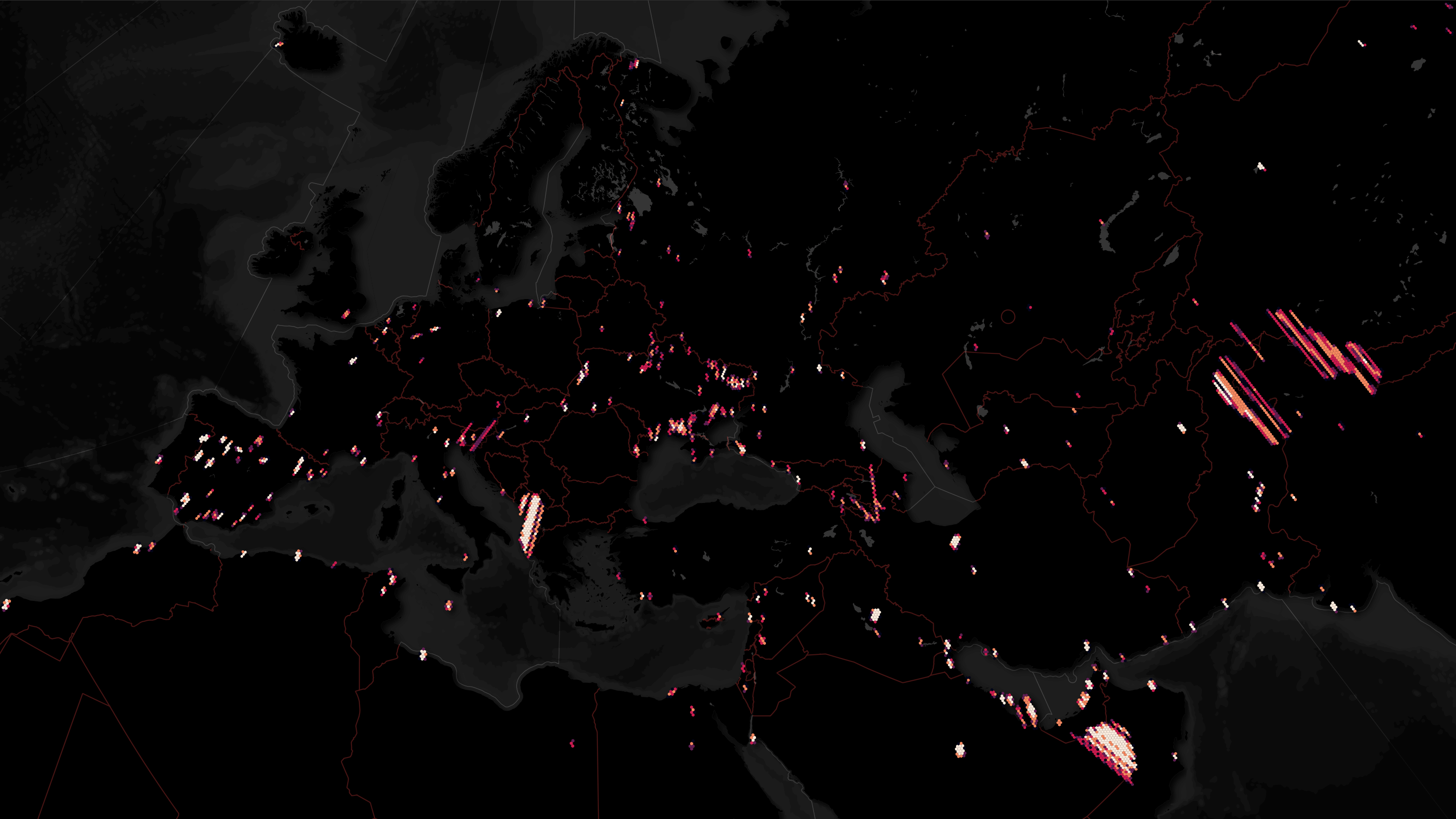
The image below might be a bit easier to see on a mobile device.

Imagery by Country
I'll use the Database of Global Administrative Areas (GADM) to get the number of images per country in this dataset.
$ wget -c https://geodata.ucdavis.edu/gadm/gadm4.1/gadm_410-gpkg.zip
$ unzip gadm_410-gpkg.zip
$ ~/duckdb ~/satellogic.duckdb
CREATE OR REPLACE TABLE gadm AS
    FROM ST_READ('gadm_410.gpkg');
The heatmap GeoPackage (GPKG) file I produced earlier has a record count for each hexagon across the globe containing at least one image. It contains 6,122 records in total. I'll use the centroid of each hexagon to find its matching country.
CREATE OR REPLACE TABLE countries AS
    SELECT   b.COUNTRY AS country,
             SUM(a.num_recs) AS num_recs
    FROM     ST_READ('h3_5.gpkg') a
    JOIN     gadm b ON ST_CONTAINS(b.geom,
                                   ST_CENTROID(a.geom))
    GROUP BY 1;
Not every centroid landed on a polygon for any of the countries listed in GADM. It could be that the missing ~1.5M image locations are just off of the coast or out in territorial waters.
SELECT SUM(num_recs)
FROM   countries;
5,763,960
Nonetheless, the following should be representative of how often any one country features in this dataset.
FROM     countries
ORDER BY num_recs DESC;
┌────────────────────────┬──────────┐
│        country         │ num_recs │
│        varchar         │  int128  │
├────────────────────────┼──────────┤
│ United States          │   886871 │
│ Saudi Arabia           │   428122 │
│ Australia              │   423079 │
│ Spain                  │   326465 │
│ China                  │   324572 │
│ México                 │   304916 │
│ Pakistan               │   293720 │
│ Russia                 │   250520 │
│ Ukraine                │   184756 │
│ Brazil                 │   176929 │
│ Argentina              │   156790 │
│ Albania                │   115472 │
│ United Arab Emirates   │   114530 │
│ Oman                   │   102500 │
│ Bangladesh             │   101888 │
│ Iran                   │    98160 │
│ India                  │    81026 │
│ Iraq                   │    72990 │
│ Canada                 │    65153 │
│ North Korea            │    64570 │
│   ·                    │       ·  │
│   ·                    │       ·  │
│   ·                    │       ·  │
│ Haiti                  │     1519 │
│ Denmark                │     1428 │
│ Moldova                │     1384 │
│ Romania                │     1291 │
│ Mozambique             │     1217 │
│ South Korea            │     1188 │
│ Colombia               │     1139 │
│ Northern Cyprus        │     1088 │
│ Slovakia               │     1075 │
│ Indonesia              │     1070 │
│ Dominican Republic     │      717 │
│ Trinidad and Tobago    │      592 │
│ Somalia                │      563 │
│ Switzerland            │      511 │
│ Serbia                 │      472 │
│ Guam                   │      431 │
│ Cuba                   │      370 │
│ Bosnia and Herzegovina │      289 │
│ Philippines            │      263 │
│ Barbados               │      244 │
├────────────────────────┴──────────┤
│ 127 rows (40 shown)     2 columns │
└───────────────────────────────────┘
Metadata and Imagery
Every image has a metadata file that describes its location, image structure and metrics around how it was captured. This file will also contain the URLs of each variation of the image, including thumbnails and the highest quality image available, which is suffed with "_VISUAL.tif".
Below is an example metadata file.
$ aws s3 cp --no-sign-request \
    s3://satellogic-earthview/data/json/zone=04N/region=603411_2346301/date=2022-09-15/20220915_010014_SN20_04N_603411_2346301_metadata.json ./

$ jq -S . 20220915_010014_SN20_04N_603411_2346301_metadata.json
{
  "assets": {
    "analytic": {
      "eo:bands": [
        {
          "common_name": "red",
          "name": "Red"
        },
        {
          "common_name": "green",
          "name": "Green"
        },
        {
          "common_name": "blue",
          "name": "Blue"
        },
        {
          "common_name": "nir",
          "name": "NIR"
        }
      ],
      "href": "https://satellogic-earthview.s3.us-west-2.amazonaws.com/data/tif/zone=04N/region=603411_2346301/date=2022-09-15/20220915_010014_SN20_04N_603411_2346301_TOA.tif",
      "roles": [
        "data",
        "reflectance"
      ],
      "type": "image/tiff; application=geotiff; profile=cloud-optimized"
    },
    "preview": {
      "href": "https://satellogic-earthview.s3.us-west-2.amazonaws.com/data/png/zone=04N/region=603411_2346301/date=2022-09-15/20220915_010014_SN20_04N_603411_2346301_preview.png",
      "roles": [
        "overview"
      ],
      "type": "image/png"
    },
    "thumbnail": {
      "href": "https://satellogic-earthview.s3.us-west-2.amazonaws.com/data/png/zone=04N/region=603411_2346301/date=2022-09-15/20220915_010014_SN20_04N_603411_2346301_thumbnail.png",
      "roles": [
        "thumbnail"
      ],
      "type": "image/png"
    },
    "visual": {
      "eo:bands": [
        {
          "common_name": "red",
          "name": "Red"
        },
        {
          "common_name": "green",
          "name": "Green"
        },
        {
          "common_name": "blue",
          "name": "Blue"
        },
        {
          "common_name": "nir",
          "name": "NIR"
        }
      ],
      "href": "https://satellogic-earthview.s3.us-west-2.amazonaws.com/data/tif/zone=04N/region=603411_2346301/date=2022-09-15/20220915_010014_SN20_04N_603411_2346301_VISUAL.tif",
      "roles": [
        "data",
        "visual"
      ],
      "type": "image/tiff; application=geotiff; profile=cloud-optimized"
    }
  },
  "bbox": [
    -158.00360706174618,
    21.211807250957015,
    -157.9998841750412,
    21.21529819598024
  ],
  "geometry": {
    "coordinates": [
      [
        [
          -157.99990754402126,
          21.211807250957015
        ],
        [
          -157.9998841750412,
          21.21527632148101
        ],
        [
          -158.00358377917712,
          21.21529819598024
        ],
        [
          -158.00360706174618,
          21.211829121542312
        ],
        [
          -157.99990754402126,
          21.211807250957015
        ]
      ]
    ],
    "type": "Polygon"
  },
  "id": "20220915_010014_SN20_04N_603411_2346301",
  "links": [
    {
      "href": "https://satellogic-earthview.s3.us-west-2.amazonaws.com/stac/2022/2022-09/2022-09-15/catalog.json",
      "rel": "parent",
      "type": "application/json"
    },
    {
      "href": "https://satellogic-earthview.s3.us-west-2.amazonaws.com/stac/catalog.json",
      "rel": "root",
      "type": "application/json"
    },
    {
      "href": "https://satellogic-earthview.s3.us-west-2.amazonaws.com/data/json/zone=04N/region=603411_2346301/date=2022-09-15/20220915_010014_SN20_04N_603411_2346301_metadata.json",
      "rel": "self",
      "type": "application/geo+json"
    }
  ],
  "properties": {
    "datetime": "2022-09-15T01:00:14.573735+00:00",
    "grid:code": "04N-603411_2346301",
    "gsd": 1,
    "license": "CC-BY-4.0",
    "platform": "newsat20",
    "proj:epsg": "32604",
    "proj:shape": [
      384,
      384
    ],
    "proj:transform": [
      1,
      0,
      603411,
      0,
      -1,
      2346301,
      0,
      0,
      1
    ],
    "providers": [
      {
        "name": "Satellogic",
        "roles": [
          "processor",
          "producer",
          "licensor"
        ],
        "url": "https://www.satellogic.com"
      },
      {
        "description": "AWS Open Data Sponsorship Program, hosting the dataset.",
        "name": "Amazon Web Services",
        "roles": [
          "host"
        ],
        "url": "https://registry.opendata.aws/"
      }
    ],
    "satl:altitude": 456.8651464515633,
    "satl:altitude_units": "km",
    "satl:product_name": "L1",
    "view:azimuth": 97.1382808902086,
    "view:off_nadir": 19.474754820772176,
    "view:sun_azimuth": 249.34650770444287,
    "view:sun_elevation": 48.67771372102758
  },
  "stac_extensions": [
    "https://stac-extensions.github.io/projection/v1.1.0/schema.json",
    "https://stac-extensions.github.io/eo/v1.1.0/schema.json",
    "https://stac-extensions.github.io/view/v1.0.0/schema.json",
    "https://stac-extensions.github.io/grid/v1.1.0/schema.json"
  ],
  "stac_version": "1.0.0",
  "type": "Feature"
}
The images themselves can be downloaded via HTTPS with no authentication.
$ wget "https://satellogic-earthview.s3.us-west-2.amazonaws.com/data/tif/zone=04N/region=603411_2346301/date=2022-09-15/20220915_010014_SN20_04N_603411_2346301_VISUAL.tif"
Qatari Imagery
I drew a bounding box around Qatar to see how many images in this dataset feature the country. Due to the country's shape and proximity to Bahrain and Saudi Arabia, a few of their images were also included in this count.
$ ~/duckdb ~/satellogic.duckdb
SELECT COUNT(*)
FROM   s3
WHERE  ST_X(geom) BETWEEN 50.6515 AND 51.8086
AND    ST_Y(geom) BETWEEN 24.3595 AND 26.3612;
┌──────────────┐
│ count_star() │
│    int64     │
├──────────────┤
│        64375 │
└──────────────┘
I'll get the URLs of the metadata for those 64,375 images and download them using eight threads.
$ echo "SELECT Key
        FROM   s3
        WHERE  ST_X(geom) BETWEEN 50.6515 AND 51.8086
        AND    ST_Y(geom) BETWEEN 24.3595 AND 26.3612" \
        | ~/duckdb -csv -noheader ~/satellogic.duckdb \
        > manifest.txt
$ mkdir qatar
$ cd qatar

$ cat ../manifest.txt \
    | xargs \
        -P8 \
        -I% \
        wget -c "https://satellogic-earthview.s3.us-west-2.amazonaws.com/%"
The above downloaded 252 MB of JSON and took almost an hour to complete. I'll concatenate those files into a single line-delimited JSON file. I'll then use DuckDB to convert the JSON into a GPKG file with a few fields cleaned up for the sake of ergonomics.
$ cd ../
$ find qatar/ \
    -type f \
    -exec cat {} + \
    > qatar.json
$ ~/duckdb
COPY (
    SELECT properties.* EXCLUDE(providers,
                                "proj:shape",
                                "proj:transform"),
           assets.preview.href          AS url_preview,
           assets.visual.href           AS url_visual,
           assets.analytic.href         AS url_analytic,
           assets.thumbnail.href        AS url_thumbnail,
           ST_GEOMFROMGEOJSON(geometry) AS geom
    FROM   'qatar.json'
) TO 'qatar.footprints.gpkg'
    WITH (FORMAT GDAL,
          DRIVER 'GPKG',
          LAYER_CREATION_OPTIONS 'WRITE_BBOX=YES');
Below is an example record of the above GPKG file.
$ echo "FROM  ST_READ('qatar.footprints.gpkg')
        LIMIT 1" \
    | ~/duckdb -json \
    | jq -S .
[
  {
    "datetime": "2022-07-14T11:06:22.192899+00:00",
    "geom": "POLYGON ((50.65626187904185 26.24828637962653, 50.656251675908884 26.25175366324302, 50.65240649343577 26.25174441056527, 50.652416810695826 26.24827712835427, 50.65626187904185 26.24828637962653))",
    "grid:code": "39N-465288_2903610",
    "gsd": 1,
    "license": "CC-BY-4.0",
    "platform": "newsat21",
    "proj:epsg": "32639",
    "satl:altitude": 461.4741909855675,
    "satl:altitude_units": "km",
    "satl:product_name": "L1",
    "url_analytic": "https://satellogic-earthview.s3.us-west-2.amazonaws.com/data/tif/zone=39N/region=465288_2903610/date=2022-07-14/20220714_110622_SN21_39N_465288_2903610_TOA.tif",
    "url_preview": "https://satellogic-earthview.s3.us-west-2.amazonaws.com/data/png/zone=39N/region=465288_2903610/date=2022-07-14/20220714_110622_SN21_39N_465288_2903610_preview.png",
    "url_thumbnail": "https://satellogic-earthview.s3.us-west-2.amazonaws.com/data/png/zone=39N/region=465288_2903610/date=2022-07-14/20220714_110622_SN21_39N_465288_2903610_thumbnail.png",
    "url_visual": "https://satellogic-earthview.s3.us-west-2.amazonaws.com/data/tif/zone=39N/region=465288_2903610/date=2022-07-14/20220714_110622_SN21_39N_465288_2903610_VISUAL.tif",
    "view:azimuth": 97.95684658243894,
    "view:off_nadir": 9.250787005630361,
    "view:sun_azimuth": 269.67692021214305,
    "view:sun_elevation": 57.10934720889825
  }
]
Below are the footprints of those 64,375 images. I've colour-coded them by the date of their capture. I've tinted the basemap blue to help the footprints stand out. The red bounding box was the search area.
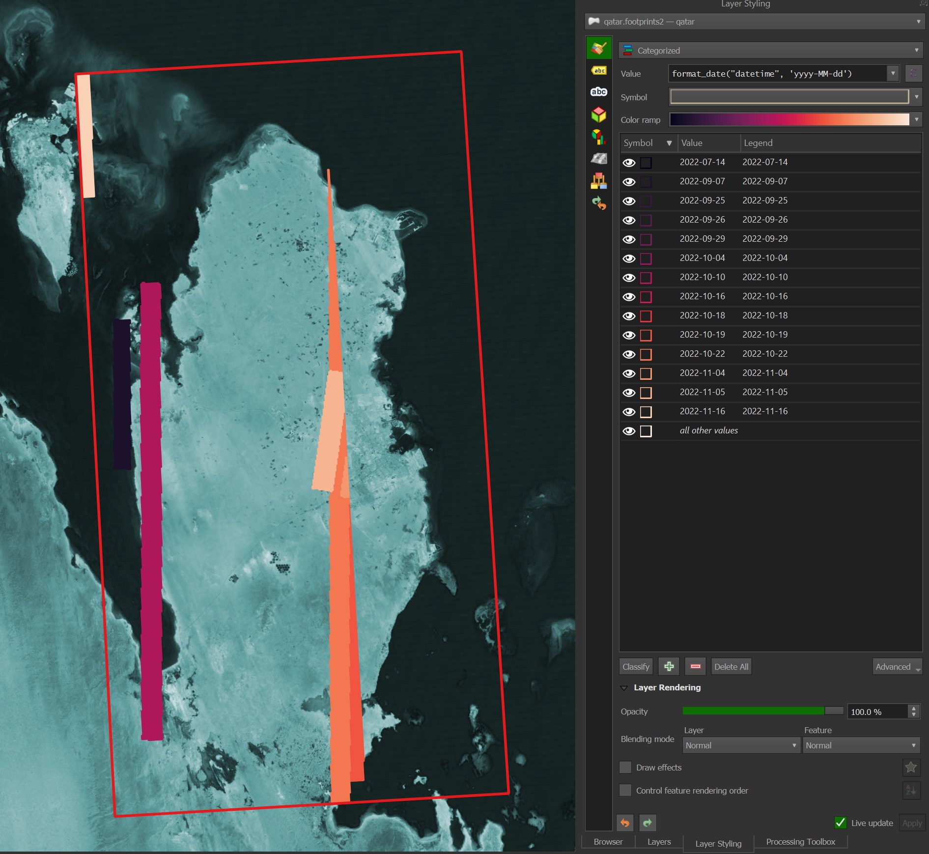
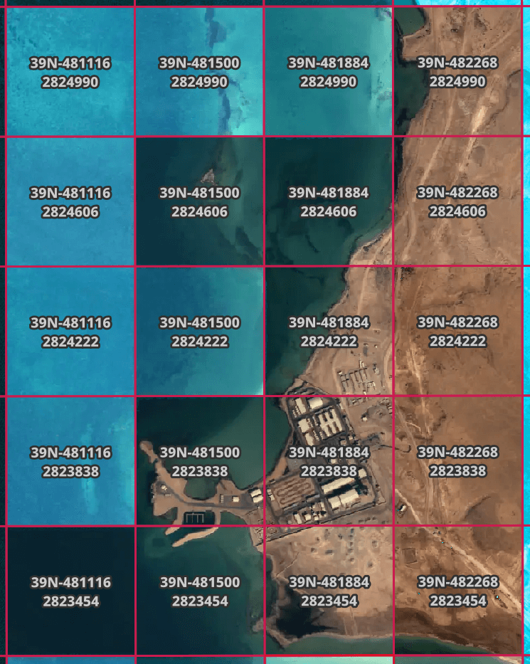
When I zoom in on any one of the large stripes of footprints, the individual footprints of each image can be seen.
I'll pick a small part of Qatar along its coastline and download that area's images.
$ echo "SELECT url_visual
        FROM   ST_READ('qatar.footprints.gpkg')
        WHERE  ST_X(ST_CENTROID(geom)) BETWEEN 50.811115 AND 50.829002
        AND    ST_Y(ST_CENTROID(geom)) BETWEEN 25.522661 AND 25.542736" \
        | ~/duckdb -csv -noheader \
        > url_visual.txt

$ mkdir imagery
$ cd imagery

$ cat ../url_visual.txt \
    | xargs \
        -P8 \
        -I% \
        wget -c "%"
The above downloaded 24 GeoTIFFs totalling 9.1 MB. Each image is 384x384-pixels.
Each image has geospatial information embedded within it, so I can group them together into a single image that will retain the spatial data. I'll re-compress the image using WebP, so the resulting image is much smaller than the original source imagery.
$ gdalbuildvrt mosaic.vrt *VISUAL.tif

$ gdal_translate \
    -co NUM_THREADS=ALL_CPUS \
    -of COG \
    -co COMPRESS=WEBP \
    -co PREDICTOR=2 \
    mosaic.vrt \
    mosaic.tif
The resulting mosaic GeoTIFF is 225 KB.
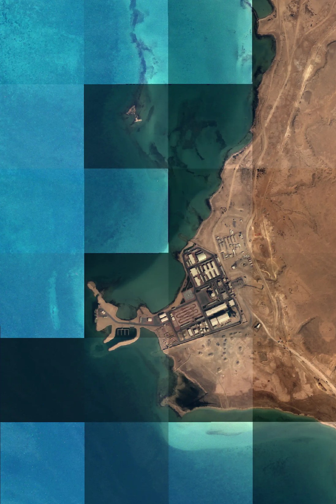
The 24 images look very different from one another and don't blend seamlessly. They share the same processing level and capture statistics, as far as I can tell.
.mode line

SELECT   datetime,
         platform,
         "satl:product_name",
         "view:azimuth",
         "view:off_nadir",
         "view:sun_azimuth",
         "view:sun_elevation",
         COUNT(*)
FROM     ST_READ('qatar.footprints.gpkg')
WHERE    ST_X(ST_CENTROID(geom)) BETWEEN 50.811115 AND 50.829002
AND      ST_Y(ST_CENTROID(geom)) BETWEEN 25.522661 AND 25.542736
GROUP BY 1, 2, 3, 4, 5, 6, 7;
          datetime = 2022-10-10T07:11:56.894566+00:00
          platform = newsat16
 satl:product_name = L1
      view:azimuth = 283.5615135582265
    view:off_nadir = 23.243003077262802
  view:sun_azimuth = 149.1609429350105
view:sun_elevation = 53.39441361193675
      count_star() = 24
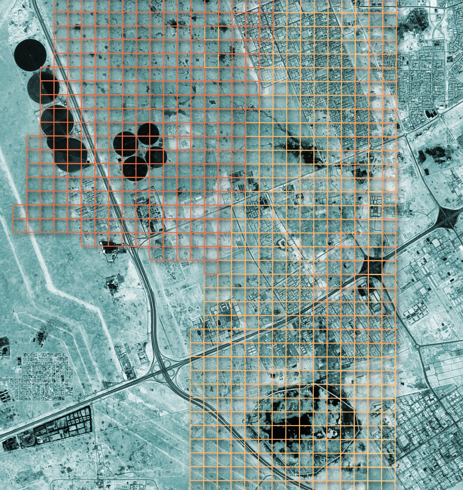
For clarity, below are the grid codes for each image in the mosaic.
The following are types of imagery deliverables that Satellogic offers:
- L0: Raw
- L1A: Raw corrected
- L1B: L1 Basic (Cloud, shadow and usable data mask)
- L1C: Ortho ready
- L1D/L1D_SR: Ortho
- L1: TOA Reflectance
- L1_SR: TOA Reflectance SuperResolution
The product listed in the metadata for these images was L1 which I'm assuming means "Radiometric-corrected imagery (TOA reflectance imagery)". Their product documentation says the imagery is corrected for sensor, optical and terrain distortions (orthorectified).
My best guess is that the images have been processed independently of one another. Basemap producers often strive to blend images next to one another seamlessly but that might not be a requirement for this imagery's original deliverable.
Cloud-Native Metadata
Last August, the Cloud-Native Geospatial Forum published an introduction to STAC GeoParquet. The post was authored by Tom Augspurger, whom has since taken on a role at Nvidia, Kyle Barron from Development Seed and Chris Holmes from Planet Labs. The STAC GeoParquet aims to optimise the storage of SpatioTemporal Asset Catalogs (STAC) metadata in GeoParquet format.
After my initial publication of this post, Brendan McAndrew downloaded all 22 GB of uncompressed JSON metadata from Satellogic and produced a GeoParquet-formatted STAC catalog. Brendan spent four years at NASA before becoming a Geospatial Software Engineer for Impact Observatory in Washington, DC.
This STAC GeoParquet file is orders of magnitude smaller than the original JSON at only 275 MB.
This file can also be downloaded much faster than the individual ~7M JSON files. The 64,375 JSON files for Qatar that I downloaded were only a few hundred MB but took over an hour to download with all the networking overhead. I was able to download this file at 28 MB/s on my 500 Mbps fiber connection.
DuckDB is also able to download individual columns of data from S3 without reading the entire file. Below I only need to download 783 KB of data out of the 275 MB file to produce a statistic on one of the columns.
$ ~/duckdb
EXPLAIN ANALYZE
    SELECT MIN(stac_version)
    FROM   READ_PARQUET('s3://satellogic-earthview-stac-geoparquet/satellogic-earthview-stac-items.parquet');
┌─────────────────────────────────────┐
│┌───────────────────────────────────┐│
││         HTTPFS HTTP Stats         ││
││                                   ││
││           in: 783.0 KiB           ││
││            out: 0 bytes           ││
││              #HEAD: 1             ││
││             #GET: 111             ││
││              #PUT: 0              ││
││              #POST: 0             ││
│└───────────────────────────────────┘│
└─────────────────────────────────────┘
┌────────────────────────────────────────────────┐
│┌──────────────────────────────────────────────┐│
││               Total Time: 1.79s              ││
│└──────────────────────────────────────────────┘│
└────────────────────────────────────────────────┘
┌───────────────────────────┐
│           QUERY           │
└─────────────┬─────────────┘
┌─────────────┴─────────────┐
│      EXPLAIN_ANALYZE      │
│    ────────────────────   │
│           0 Rows          │
│          (0.00s)          │
└─────────────┬─────────────┘
┌─────────────┴─────────────┐
│    UNGROUPED_AGGREGATE    │
│    ────────────────────   │
│    Aggregates: min(#0)    │
│                           │
│           1 Rows          │
│          (0.05s)          │
└─────────────┬─────────────┘
┌─────────────┴─────────────┐
│         PROJECTION        │
│    ────────────────────   │
│        stac_version       │
│                           │
│        7095985 Rows       │
│          (0.00s)          │
└─────────────┬─────────────┘
┌─────────────┴─────────────┐
│         TABLE_SCAN        │
│    ────────────────────   │
│         Function:         │
│        READ_PARQUET       │
│                           │
│        Projections:       │
│        stac_version       │
│                           │
│        7095985 Rows       │
│          (51.22s)         │
└───────────────────────────┘
Below is an example record from Brendan's version of Satellogic's metadata.
$ echo "SELECT * EXCLUDE(assets,
                         links,
                         providers,
                         stac_extensions),
               assets::JSON assets,
               links::JSON links,
               providers::JSON providers,
               stac_extensions::JSON stac_extensions
        FROM READ_PARQUET('s3://satellogic-earthview-stac-geoparquet/satellogic-earthview-stac-items.parquet')
      LIMIT 1" \
    | ~/duckdb -json \
    | jq -S .
[
  {
    "assets": {
      "analytic": {
        "eo:bands": [
          {
            "common_name": "red",
            "name": "Red"
          },
          {
            "common_name": "green",
            "name": "Green"
          },
          {
            "common_name": "blue",
            "name": "Blue"
          },
          {
            "common_name": "nir",
            "name": "NIR"
          }
        ],
        "href": "https://satellogic-earthview.s3.us-west-2.amazonaws.com/data/tif/zone=21S/region=667983_6954390/date=2022-07-01/20220701_142509_SN23_21S_667983_6954390_TOA.tif",
        "roles": [
          "data",
          "reflectance"
        ],
        "type": "image/tiff; application=geotiff; profile=cloud-optimized"
      },
      "preview": {
        "href": "https://satellogic-earthview.s3.us-west-2.amazonaws.com/data/png/zone=21S/region=667983_6954390/date=2022-07-01/20220701_142509_SN23_21S_667983_6954390_preview.png",
        "roles": [
          "overview"
        ],
        "type": "image/png"
      },
      "thumbnail": {
        "href": "https://satellogic-earthview.s3.us-west-2.amazonaws.com/data/png/zone=21S/region=667983_6954390/date=2022-07-01/20220701_142509_SN23_21S_667983_6954390_thumbnail.png",
        "roles": [
          "thumbnail"
        ],
        "type": "image/png"
      },
      "visual": {
        "eo:bands": [
          {
            "common_name": "red",
            "name": "Red"
          },
          {
            "common_name": "green",
            "name": "Green"
          },
          {
            "common_name": "blue",
            "name": "Blue"
          },
          {
            "common_name": "nir",
            "name": "NIR"
          }
        ],
        "href": "https://satellogic-earthview.s3.us-west-2.amazonaws.com/data/tif/zone=21S/region=667983_6954390/date=2022-07-01/20220701_142509_SN23_21S_667983_6954390_VISUAL.tif",
        "roles": [
          "data",
          "visual"
        ],
        "type": "image/tiff; application=geotiff; profile=cloud-optimized"
      }
    },
    "bbox": "{'xmin': -55.29907329132605, 'ymin': -27.52730527848537, 'xmax': -55.29513299608709, 'ymax': -27.523792485602513}",
    "datetime": "2022-07-01 17:25:09.03115+03",
    "geometry": "POLYGON ((-55.29513299608709 -27.52725766492321, -55.29518646111154 -27.523792485602513, -55.29907329132605 -27.523840092170495, -55.29901994805388 -27.52730527848537, -55.29513299608709 -27.52725766492321))",
    "grid:code": "21S-667983_6954390",
    "gsd": 1.0,
    "id": "20220701_142509_SN23_21S_667983_6954390",
    "license": "CC-BY-4.0",
    "links": [
      {
        "href": "https://satellogic-earthview.s3.us-west-2.amazonaws.com/stac/2022/2022-07/2022-07-01/catalog.json",
        "rel": "parent",
        "type": "application/json"
      },
      {
        "href": "https://satellogic-earthview.s3.us-west-2.amazonaws.com/stac/catalog.json",
        "rel": "root",
        "type": "application/json"
      },
      {
        "href": "https://satellogic-earthview.s3.us-west-2.amazonaws.com/data/json/zone=21S/region=667983_6954390/date=2022-07-01/20220701_142509_SN23_21S_667983_6954390_metadata.json",
        "rel": "self",
        "type": "application/geo+json"
      }
    ],
    "platform": "newsat23",
    "proj:epsg": "32721",
    "proj:shape": "[384, 384]",
    "proj:transform": "[1.0, 0.0, 667983.0, 0.0, -1.0, 6954390.0, 0.0, 0.0, 1.0]",
    "providers": [
      {
        "description": null,
        "name": "Satellogic",
        "roles": [
          "processor",
          "producer",
          "licensor"
        ],
        "url": "https://www.satellogic.com"
      },
      {
        "description": "AWS Open Data Sponsorship Program, hosting the dataset.",
        "name": "Amazon Web Services",
        "roles": [
          "host"
        ],
        "url": "https://registry.opendata.aws/"
      }
    ],
    "satl:altitude": 514.0430664434643,
    "satl:altitude_units": "km",
    "satl:product_name": "L1",
    "stac_extensions": [
      "https://stac-extensions.github.io/projection/v1.1.0/schema.json",
      "https://stac-extensions.github.io/eo/v1.1.0/schema.json",
      "https://stac-extensions.github.io/view/v1.0.0/schema.json",
      "https://stac-extensions.github.io/grid/v1.1.0/schema.json"
    ],
    "stac_version": "1.0.0",
    "type": "Feature",
    "view:azimuth": 286.1475475384163,
    "view:off_nadir": 8.171090276284483,
    "view:sun_azimuth": 22.808714817358606,
    "view:sun_elevation": 35.85325119151129
  }
]
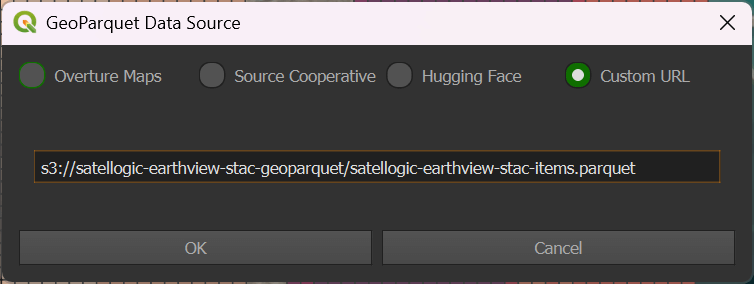
GeoParquet Downloader for QGIS
Chris Holmes has been working on a QGIS plugin for the past few months called GeoParquet Downloader for QGIS. I've opened QGIS, added a world map and zoomed into Bahrain. Chris' plug-in will use the bounding box of the viewport to isolate records for that area.
I've launched Chris' plug-in, selected "Custom URL" and pasted the following URL in.
s3://satellogic-earthview-stac-geoparquet/satellogic-earthview-stac-items.parquet
Now I'm able to see polygon footprints for each image in Satellogic's dataset just for Bahrain. Chris' plug-in only had to download 460 KB of data from the 275 MB file on S3.
Clicking on any one footprint with the "Identify Features" tool will display their respective metadata.
Below I've colour-coded the footprints based on their capture date.
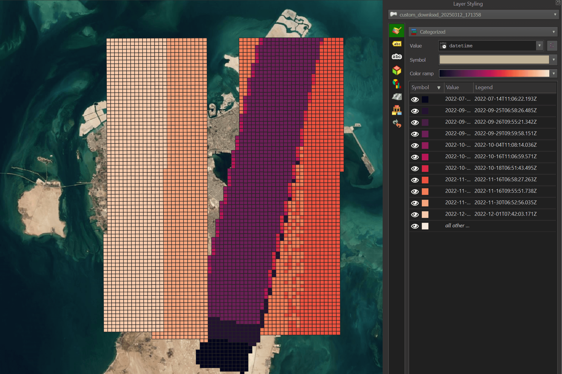
Below I've grouped the image footprints by month, set the blend mode to hard light, sorted the render order by date and added a drop shadow effect. As I enable each layer for each month, their overlapping footprints are clear to see.
