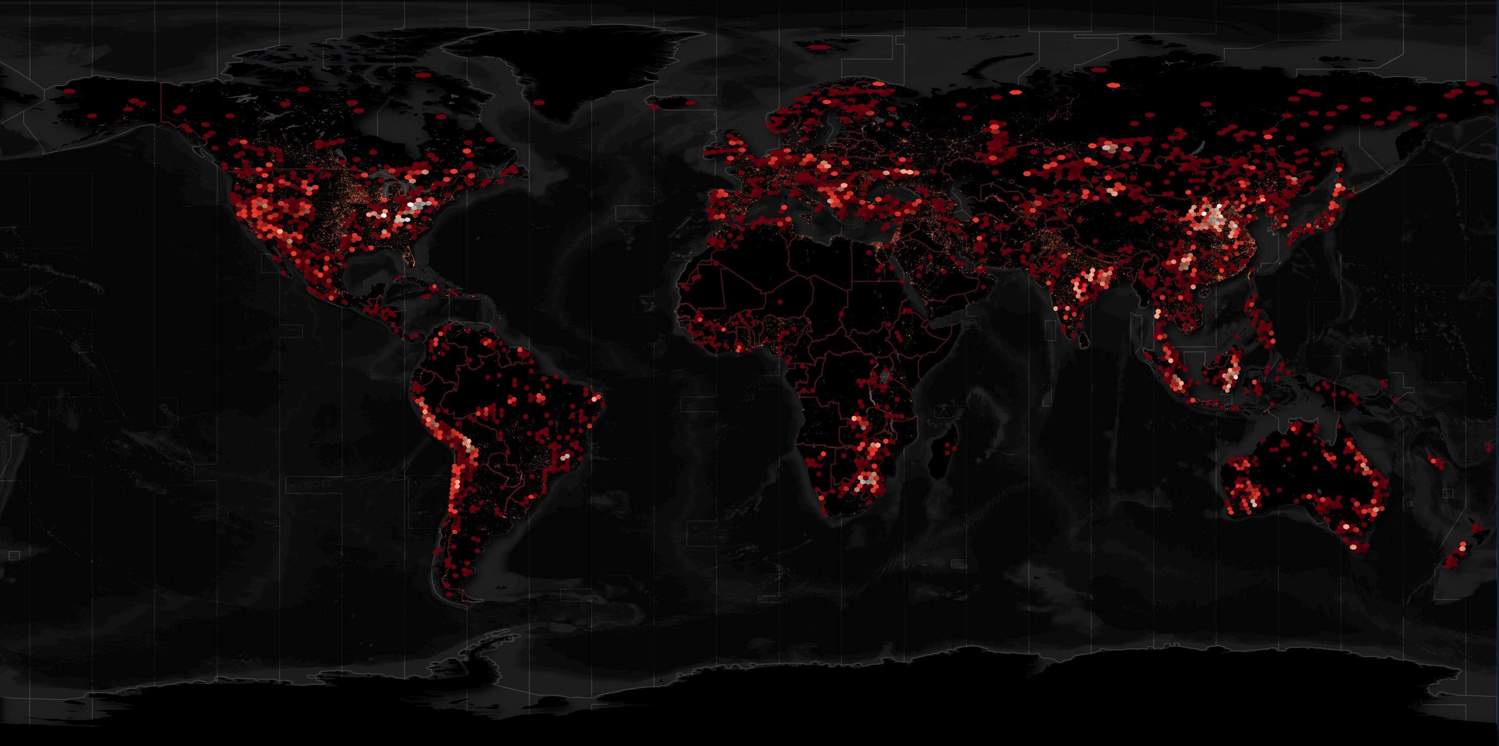
The International Council on Mining and Metals (ICMM) is a mining industry group that was founded in London in 2001. In September, they released a Global Mining Dataset containing over 8,000 mines and other related assets around the globe.
Below is a heatmap of the assets they catalogued in this dataset.
In this post, I'll explore ICMM's mining dataset.
My Workstation
I'm using a 5.7 GHz AMD Ryzen 9 9950X CPU. It has 16 cores and 32 threads and 1.2 MB of L1, 16 MB of L2 and 64 MB of L3 cache. It has a liquid cooler attached and is housed in a spacious, full-sized Cooler Master HAF 700 computer case.
The system has 96 GB of DDR5 RAM clocked at 4,800 MT/s and a 5th-generation, Crucial T700 4 TB NVMe M.2 SSD which can read at speeds up to 12,400 MB/s. There is a heatsink on the SSD to help keep its temperature down. This is my system's C drive.
The system is powered by a 1,200-watt, fully modular Corsair Power Supply and is sat on an ASRock X870E Nova 90 Motherboard.
I'm running Ubuntu 24 LTS via Microsoft's Ubuntu for Windows on Windows 11 Pro. In case you're wondering why I don't run a Linux-based desktop as my primary work environment, I'm still using an Nvidia GTX 1080 GPU which has better driver support on Windows and ArcGIS Pro only supports Windows natively.
Installing Prerequisites
I'll use Python 3.12.3 and a few other tools to help analyse the data in this post.
$ sudo add-apt-repository ppa:deadsnakes/ppa
$ sudo apt update
$ sudo apt install \
    jq \
    python3-pip \
    python3.12-venv
I'll set up a Python Virtual Environment and install an OSM vector tile data extraction utility I wrote last year.
$ python3 -m venv ~/.osm
$ source ~/.osm/bin/activate

$ git clone https://github.com/marklit/tiles2columns \
    ~/tiles2columns
$ python -m pip install \
         -r ~/tiles2columns/requirements.txt
I'll use DuckDB v1.3.0, along with its H3, JSON, Lindel, Parquet and Spatial extensions, in this post. Normally I try and use the latest release of DuckDB but v1.4.0 has an issue where it's Parquet files aren't readable by many of the tools I use at the moment.
$ cd ~
$ wget -c https://github.com/duckdb/duckdb/releases/download/v1.3.0/duckdb_cli-linux-amd64.zip
$ unzip -j duckdb_cli-linux-amd64.zip
$ chmod +x duckdb
$ ~/duckdb
INSTALL h3 FROM community;
INSTALL lindel FROM community;
INSTALL json;
INSTALL parquet;
INSTALL spatial;
I'll set up DuckDB to load every installed extension each time it launches.
$ vi ~/.duckdbrc
.timer on
.width 180
LOAD h3;
LOAD lindel;
LOAD json;
LOAD parquet;
LOAD spatial;
The maps in this post were mostly rendered with QGIS version 3.44. QGIS is a desktop application that runs on Windows, macOS and Linux. The application has grown in popularity in recent years and has ~15M application launches from users all around the world each month.
I used QGIS' Tile+ plugin to add basemaps from Esri to one of the maps in this post.
The dark, non-satellite map of ICMM's asset locations above is mostly made up of vector data from Natural Earth and Overture.
Analysis-Ready Data
I'll download ICMM's Excel file for this dataset.
$ wget -O global-mining-dataset.xlsx \
    'https://www.icmm.com/website/data/2025/global-mining-dataset.xlsx?cb=117612'
I'll use DuckDB to clean up the values and produce both a geometry field and a bounding box for each feature in this dataset. This will make working with this dataset remotely, such as from AWS S3, much easier.
$ ~/duckdb
CREATE OR REPLACE TABLE icmm AS
    SELECT * EXCLUDE(Latitude,
                     Longitude,
                     "Mine Name",
                     "Primary Commodity",
                     "Secondary Commodity",
                     "Other Commodities"),
           ST_POINT(Longitude, Latitude) AS geometry,
           {'xmin': ST_XMIN(ST_EXTENT(geometry)),
            'ymin': ST_YMIN(ST_EXTENT(geometry)),
            'xmax': ST_XMAX(ST_EXTENT(geometry)),
            'ymax': ST_YMAX(ST_EXTENT(geometry))} AS bbox,
           TRIM("Mine Name")           AS "Mine Name",
           TRIM("Primary Commodity")   AS "Primary Commodity",
           TRIM("Secondary Commodity") AS "Secondary Commodity"
    FROM READ_XLSX('global-mining-dataset.xlsx',
                   sheet='External',
                   ignore_errors=true);
This following produced a ZStandard-compressed, spatially-sorted Parquet file of ICMM's dataset.
COPY (
    SELECT   * EXCLUDE (geometry),
             ST_ASWKB(geometry) geometry
    FROM     icmm
    WHERE    ST_X(ST_CENTROID(geometry)) IS NOT NULL
    ORDER BY HILBERT_ENCODE([ST_Y(ST_CENTROID(geometry)),
                             ST_X(ST_CENTROID(geometry))]::double[2])
) TO 'icmm.parquet' (
   FORMAT            'PARQUET',
   CODEC             'ZSTD',
   COMPRESSION_LEVEL 22,
   ROW_GROUP_SIZE    15000);
Data Fluency
The above Parquet file is 508 KB and contains 8,508 rows. Below is an example record.
$ echo "SELECT * EXCLUDE(bbox),
               bbox::JSON bbox
        FROM   READ_PARQUET('icmm.parquet')
        WHERE  ICMMID = 'ICMM08147'" \
    | ~/duckdb -json \
    | jq -S .
[
  {
    "Asset Type": "Mine",
    "Confidence Factor": "High",
    "Country or Region": "Canada",
    "Group Names": "Diavik;Diavik",
    "ICMMID": "ICMM08147",
    "Mine Name": "Diavik",
    "Primary Commodity": "diamond",
    "Secondary Commodity": null,
    "bbox": {
      "xmax": -110.2743898,
      "xmin": -110.2743898,
      "ymax": 64.49236014,
      "ymin": 64.49236014
    },
    "geometry": "POINT (-110.2743898 64.49236014)"
  }
]
Below are the field names, data types, percentages of NULLs per column, number of unique values and minimum and maximum values for each column.
SELECT   column_name,
         column_type,
         null_percentage,
         approx_unique,
         min,
         max
FROM     (SUMMARIZE
          FROM icmm)
WHERE    column_name != 'geometry'
AND      column_name != 'bbox'
ORDER BY 1;
┌─────────────────────┬─────────────┬─────────────────┬───────────────┬───────────────────────┬────────────────────┐
│     column_name     │ column_type │ null_percentage │ approx_unique │          min          │        max         │
│       varchar       │   varchar   │  decimal(9,2)   │     int64     │        varchar        │      varchar       │
├─────────────────────┼─────────────┼─────────────────┼───────────────┼───────────────────────┼────────────────────┤
│ Asset Type          │ VARCHAR     │            0.00 │            17 │ Mine                  │ Steel Plant        │
│ Confidence Factor   │ VARCHAR     │            0.00 │             3 │ High                  │ Very Low           │
│ Country or Region   │ VARCHAR     │            0.00 │           129 │ Afghanistan           │ Zimbabwe           │
│ Group Names         │ VARCHAR     │           50.25 │          3639 │ # 5 Mine;No. 5 Coal…  │ ÄŒSA Coal Mine;CSA │
│ ICMMID              │ VARCHAR     │            0.00 │          7920 │ ICMM00026             │ ICMM21432          │
│ Mine Name           │ VARCHAR     │            0.00 │          8754 │ # 5 Mine              │ ÄŒSA Coal Mine     │
│ Primary Commodity   │ VARCHAR     │            0.00 │            43 │ alumina               │ zircon             │
│ Secondary Commodity │ VARCHAR     │           72.57 │            60 │ alumina               │ zircon             │
└─────────────────────┴─────────────┴─────────────────┴───────────────┴───────────────────────┴────────────────────┘
Commodities
Below is the number of assets per primary community type broken down by confidence factor.
.maxrows 100

PIVOT    READ_PARQUET('icmm.parquet')
ON       "Confidence Factor"
USING    COUNT(*)
GROUP BY "Primary Commodity"
ORDER BY "Primary Commodity";
┌────────────────────────┬───────┬──────────┬──────────┐
│   Primary Commodity    │ High  │ Moderate │ Very Low │
│        varchar         │ int64 │  int64   │  int64   │
├────────────────────────┼───────┼──────────┼──────────┤
│ alumina                │    64 │        5 │        0 │
│ aluminium              │    91 │        9 │        0 │
│ antimony               │     0 │        1 │        5 │
│ barium                 │     0 │        0 │      134 │
│ bauxite                │    17 │        5 │        0 │
│ borates                │     0 │        1 │        0 │
│ boron                  │     0 │        0 │        2 │
│ chromite               │     2 │       27 │        4 │
│ chromium               │     3 │        9 │       46 │
│ coal                   │   508 │      729 │        0 │
│ cobalt                 │     3 │        0 │       12 │
│ copper                 │   336 │      212 │      353 │
│ diamond                │     5 │        0 │        0 │
│ ferrochrome            │     0 │        2 │        0 │
│ ferromanganese         │     3 │        2 │        0 │
│ ferronickel            │     8 │        1 │        0 │
│ ferroniobium           │     0 │        1 │        0 │
│ ferrosilicon manganese │     0 │        1 │        0 │
│ fluorspar              │     0 │        1 │        0 │
│ gold                   │   379 │      261 │      237 │
│ heavy mineral sands    │     3 │        0 │        0 │
│ ilmenite               │     1 │        3 │        0 │
│ iron ore               │   299 │      312 │        0 │
│ lanthanides            │     0 │        1 │        0 │
│ lead                   │    31 │       46 │       33 │
│ lithium                │    34 │        7 │       24 │
│ manganese              │     5 │        1 │        0 │
│ mercury                │     0 │        0 │        2 │
│ metallurgical coal     │   366 │      525 │        0 │
│ molybdenum             │     2 │        1 │        0 │
│ nickel                 │    52 │       25 │       71 │
│ niobium                │     1 │        0 │        0 │
│ palladium              │     1 │        0 │        0 │
│ phosphate              │     2 │        5 │        0 │
│ platinum               │    24 │        2 │       59 │
│ potash                 │     1 │        0 │        0 │
│ silver                 │    49 │       18 │      179 │
│ steel                  │     8 │       75 │        0 │
│ thermal coal           │   675 │     1382 │        0 │
│ tin                    │     1 │       20 │      277 │
│ titanium               │     1 │        0 │        0 │
│ tungsten               │     0 │       11 │       94 │
│ uranium                │     1 │        3 │        3 │
│ vanadium               │     1 │        0 │        0 │
│ zinc                   │   183 │       18 │       89 │
│ zircon                 │     0 │        1 │        0 │
├────────────────────────┴───────┴──────────┴──────────┤
│ 46 rows                                    4 columns │
└──────────────────────────────────────────────────────┘
Below are the most common primary and secondary commodity pairs.
SELECT   "Primary Commodity",
         "Secondary Commodity",
         COUNT(*)
FROM     READ_PARQUET('icmm.parquet')
WHERE    "Secondary Commodity" IS NOT NULL
GROUP BY 1, 2
ORDER BY 3 DESC
LIMIT    50;
┌────────────────────┬─────────────────────┬──────────────┐
│ Primary Commodity  │ Secondary Commodity │ count_star() │
│      varchar       │       varchar       │    int64     │
├────────────────────┼─────────────────────┼──────────────┤
│ gold               │ silver              │          398 │
│ metallurgical coal │ thermal coal        │          396 │
│ copper             │ gold                │          361 │
│ zinc               │ lead                │          115 │
│ copper             │ silver              │           53 │
│ lead               │ zinc                │           52 │
│ gold               │ copper              │           48 │
│ copper             │ cobalt              │           44 │
│ copper             │ lead                │           40 │
│ nickel             │ cobalt              │           40 │
│ copper             │ molybdenum          │           40 │
│ silver             │ gold                │           36 │
│ nickel             │ copper              │           35 │
│ copper             │ zinc                │           28 │
│ gold               │ platinum            │           28 │
│ gold               │ lead                │           27 │
│ copper             │ nickel              │           27 │
│ silver             │ lead                │           23 │
│ lead               │ silver              │           22 │
│ zinc               │ copper              │           21 │
│ tin                │ tungsten            │           20 │
│ chromite           │ chromium            │           20 │
│ zinc               │ silver              │           20 │
│ platinum           │ palladium           │           19 │
│ alumina            │ aluminium           │           19 │
│ iron ore           │ manganese           │           17 │
│ silver             │ zinc                │           13 │
│ lithium            │ tantalum            │           11 │
│ tin                │ zinc                │           11 │
│ lead               │ copper              │           10 │
│ silver             │ copper              │           10 │
│ gold               │ palladium           │            9 │
│ steel              │ iron                │            8 │
│ gold               │ antimony            │            8 │
│ ferronickel        │ nickel              │            8 │
│ copper             │ platinum            │            8 │
│ alumina            │ bauxite             │            8 │
│ gold               │ uranium             │            7 │
│ zinc               │ cadmium             │            7 │
│ iron ore           │ copper              │            6 │
│ iron ore           │ gold                │            6 │
│ gold               │ zinc                │            6 │
│ gold               │ arsenic             │            6 │
│ lithium            │ potash              │            5 │
│ tin                │ silver              │            5 │
│ chromium           │ chromite            │            5 │
│ gold               │ iron ore            │            5 │
│ gold               │ nickel              │            5 │
│ zinc               │ gold                │            5 │
│ antimony           │ gold                │            4 │
├────────────────────┴─────────────────────┴──────────────┤
│ 50 rows                                       3 columns │
└─────────────────────────────────────────────────────────┘
Assets
This is the number of asset types in this dataset broken down by confidence factor. Some assets are the combination of two or more types.
PIVOT    READ_PARQUET('icmm.parquet')
ON       "Confidence Factor"
USING    COUNT(*)
GROUP BY "Asset Type"
ORDER BY "Asset Type";
┌────────────────────────┬───────┬──────────┬──────────┐
│       Asset Type       │ High  │ Moderate │ Very Low │
│        varchar         │ int64 │  int64   │  int64   │
├────────────────────────┼───────┼──────────┼──────────┤
│ Mine                   │  2702 │     3518 │     1576 │
│ Mine;Plant             │    68 │       48 │        7 │
│ Mine;Refinery          │    13 │        5 │        0 │
│ Mine;Refinery;Plant    │     0 │        1 │        0 │
│ Mine;Smelter           │    22 │       21 │        1 │
│ Mine;Smelter;Plant     │     3 │        3 │        0 │
│ Mine;Smelter;Refinery  │    18 │       11 │        0 │
│ Plant                  │     9 │       11 │       31 │
│ Refinery               │    59 │       16 │        1 │
│ Refinery; Steel Plant  │     1 │        0 │        0 │
│ Refinery;Plant         │     3 │        1 │        1 │
│ Smelter                │   143 │       64 │        7 │
│ Smelter;Plant          │     3 │        1 │        0 │
│ Smelter;Refinery       │   106 │        3 │        0 │
│ Smelter;Refinery;Plant │     5 │        2 │        0 │
│ Smelter;Steel Plant    │     2 │        0 │        0 │
│ Steel Plant            │     3 │       18 │        0 │
├────────────────────────┴───────┴──────────┴──────────┤
│ 17 rows                                    4 columns │
└──────────────────────────────────────────────────────┘
Countries
Below are the most and least represented countries in this dataset.
.maxrows 25

SELECT   COUNT(*),
         "Country or Region"
FROM     READ_PARQUET('icmm.parquet')
GROUP BY 2
ORDER BY 1 DESC;
┌──────────────┬─────────────────────┐
│ count_star() │  Country or Region  │
│    int64     │       varchar       │
├──────────────┼─────────────────────┤
│         1839 │ China               │
│         1627 │ United States       │
│          588 │ Australia           │
│          473 │ Indonesia           │
│          424 │ India               │
│          328 │ Russia              │
│          272 │ South Africa        │
│          252 │ Brazil              │
│          206 │ Peru                │
│          197 │ Canada              │
│          146 │ Bolivia             │
│          144 │ Chile               │
│          136 │ Mexico              │
│            · │  ·                  │
│            · │  ·                  │
│            · │  ·                  │
│            2 │ Fiji                │
│            1 │ Rwanda              │
│            1 │ Trinidad and Tobago │
│            1 │ Gabon               │
│            1 │ Bangladesh          │
│            1 │ Bahrain             │
│            1 │ Nepal               │
│            1 │ Luxembourg          │
│            1 │ Taiwan              │
│            1 │ Niger               │
│            1 │ Qatar               │
│            1 │ Greenland           │
├──────────────┴─────────────────────┤
│ 129 rows (25 shown)      2 columns │
└────────────────────────────────────┘
I'll generate a heatmap of the asset locations in this dataset.
CREATE OR REPLACE TABLE h3_3_stats AS
    SELECT   H3_LATLNG_TO_CELL(
                bbox.ymin,
                bbox.xmin, 3) AS h3_3,
             COUNT(*) num_buildings
    FROM     READ_PARQUET('icmm.parquet')
    WHERE    bbox.xmin BETWEEN -178.25 AND 178.25
    GROUP BY 1;

COPY (
    SELECT ST_ASWKB(H3_CELL_TO_BOUNDARY_WKT(h3_3)::geometry) geometry,
           num_buildings
    FROM   h3_3_stats
) TO 'h3_3_stats.gpkg'
  WITH (FORMAT GDAL,
        DRIVER 'GPKG',
        LAYER_CREATION_OPTIONS 'WRITE_BBOX=YES');
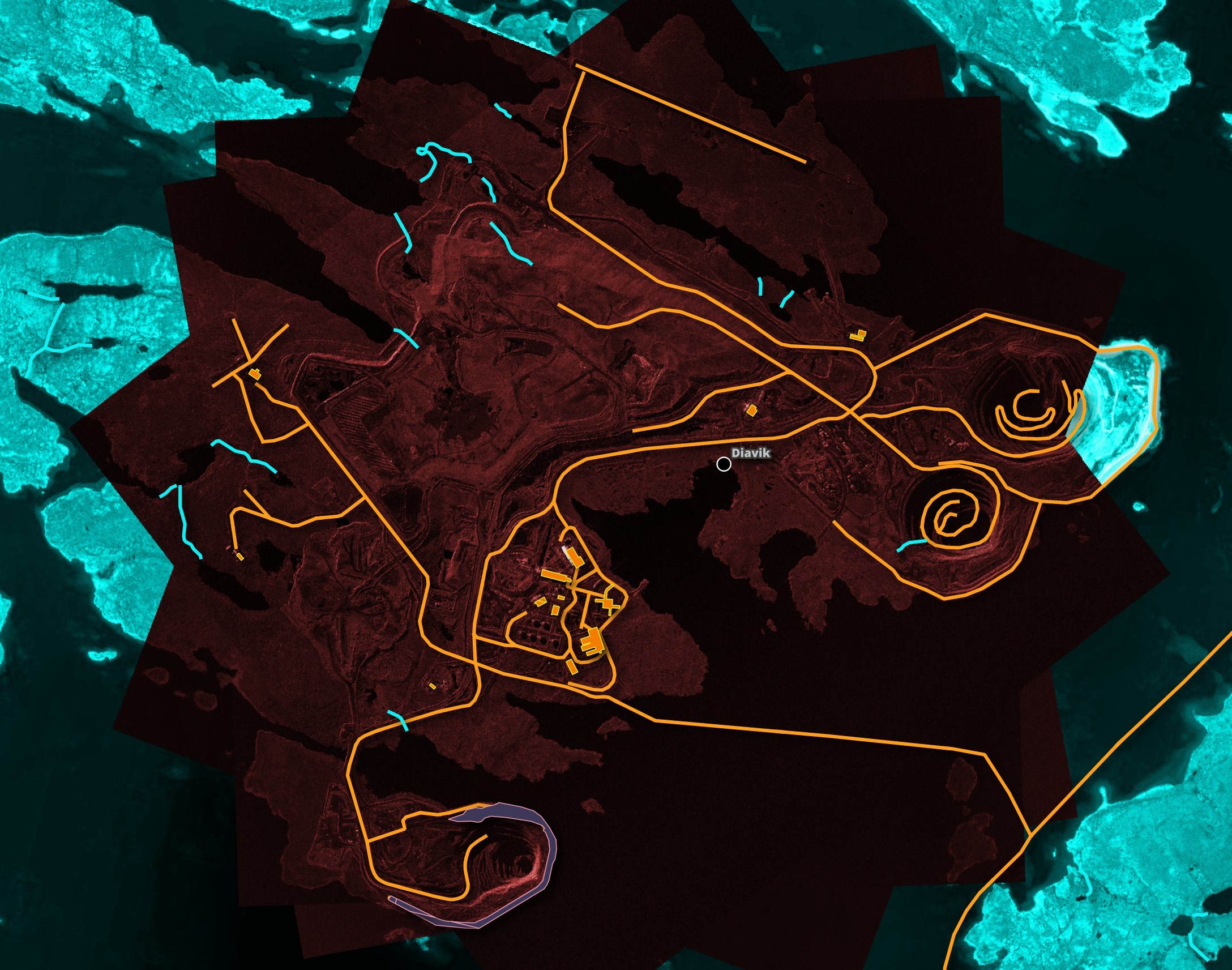
Diavik Diamond Mine
I'll download OpenStreetMap's (OSM) data for Canada's Diavik Diamond Mine. This is using the tiles2columns utility I built last year following OSM's addition of vector-based tiles to their service.
$ mkdir -p ~/diavik
$ cd ~/diavik

$ python3 ~/tiles2columns/main.py \
    centroid \
    -110.29299 64.48937 \
    --distance 0.1
The above extracted 1.2 MB worth of GeoPackage (GPKG) files. They're grouped by feature type.
$ du -hsc *
96K     buildings.gpkg
96K     dam_polygons.gpkg
124K    land.gpkg
96K     public_transport.gpkg
96K     street_labels.gpkg
128K    streets.gpkg
148K    water_lines.gpkg
404K    water_polygons.gpkg
1.2M    total
Umbra are a satellite manufacturer and constellation operator. They produce Synthetic Aperture Radar (SAR) satellites that can see through clouds and capture imagery of the earth day or night.
They operate an open feed with some of the imagery they capture. One of the locations they publish imagery of regularly is the Diavik Diamond Mine.
I've placed four images they captured on August 26th and September 5th, 17th and 26th on top of one another. Each image has a slightly different footprint so the four images in combination cover a wider area than any one image. Given how mines can change from day to day I've constrained the overlapping of imagery to a few weeks.
The image below has Esri's World Imagery basemap tinted blue. Tinted red is Umbra's imagery and the vector data on top is from OSM. I've used EPSG:3978 for the projection as this is in Northern Canada.