GeoDeep is a Python package that can detect objects in satellite imagery. It's made up of 1,026 lines of Python and uses ONNX Runtime and Rasterio extensively.
GeoDeep was written by Piero Toffanin, who is based in Florida and is the co-founder of OpenDroneMap. He also wrote LibreTranslate which I covered in a post a while back.
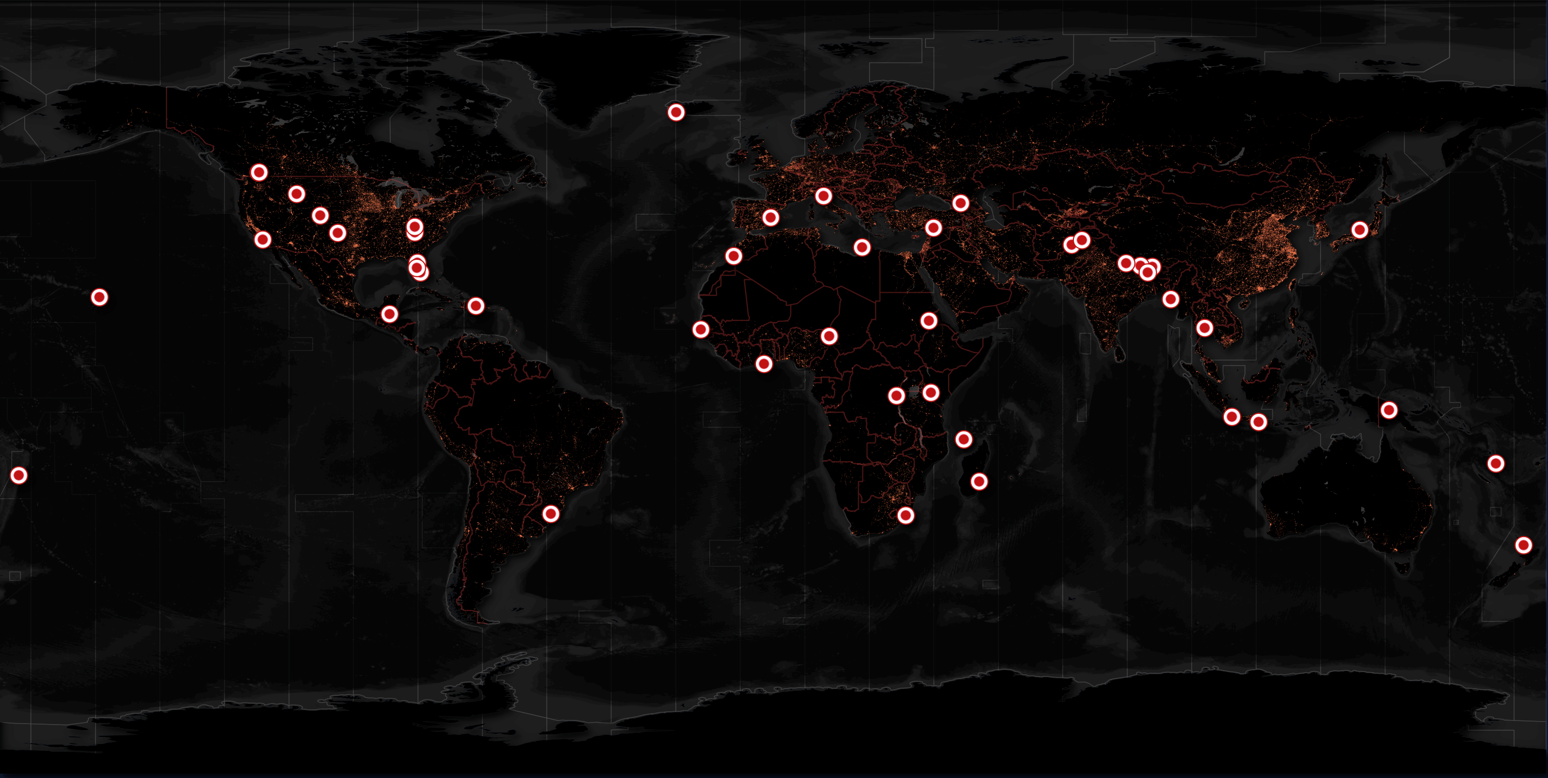
Maxar is a satellite manufacturer and constellation operator. They run an open data programme and they often releases imagery from areas before and after natural disasters strike. Below are the locations of their releases to date.
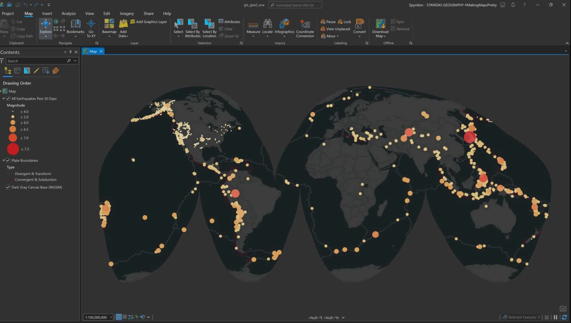
On March 28th, an earthquake struck Myanmar and it reached as far away as Bangkok, Thailand. Spyridon Staridas, a cartographer based in Greece, put together this map of earthquake history around the world. Thailand is surrounded by countries that are earthquake-prone but these are relatively rare in Thailand compared to elsewhere in Asia.
Shortly after the earthquake, Maxar released historical satellite imagery from the affected areas and later included imagery taken after the earthquake. As of this writing, they've released almost 10 GB of GeoTIFFs.
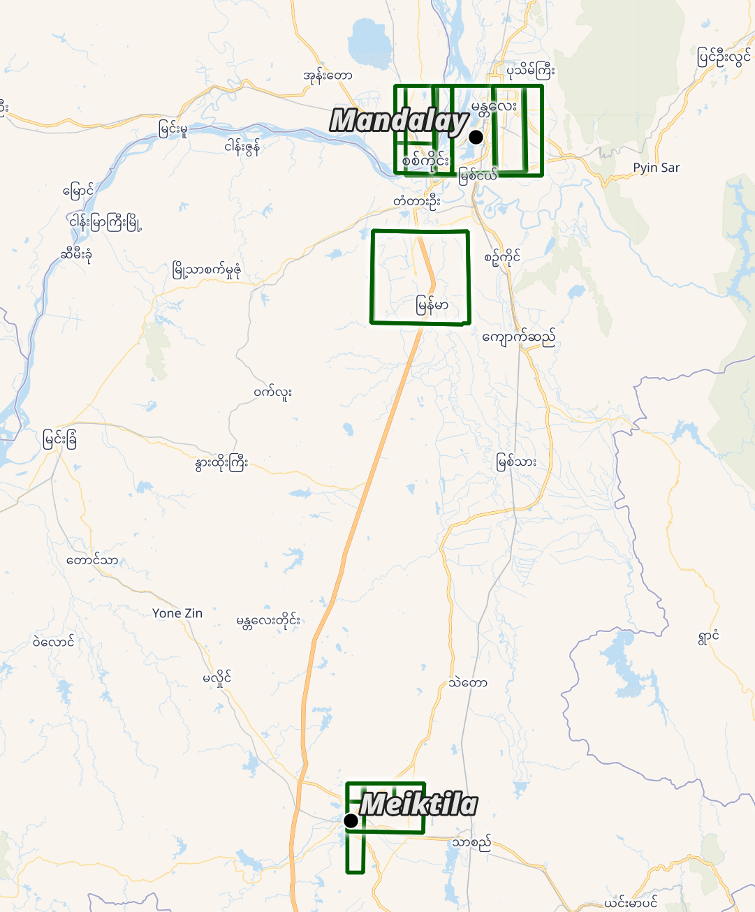
Below are the imagery footprints in central Myanmar. The imagery spans from February 2nd till early April.
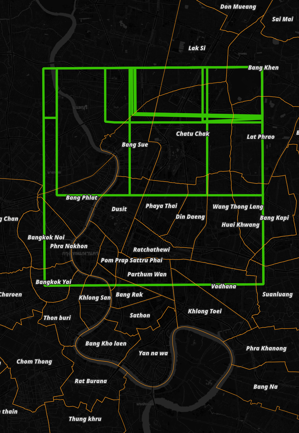
Below are the satellite footprints for Bangkok.
In this post, I'll run some of GeoDeep's built-in AI models on Maxar's satellite imagery of Myanmar and Bangkok, Thailand.
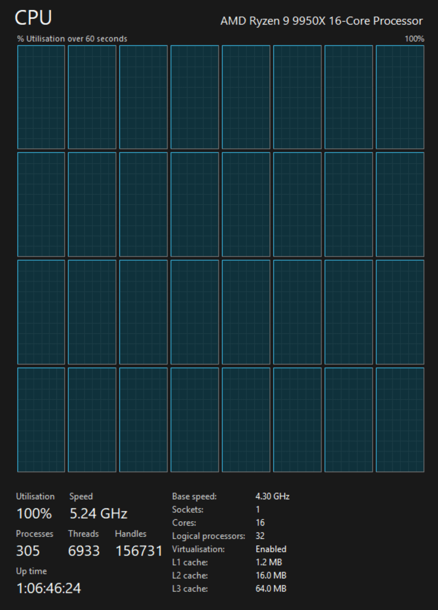
My Workstation
I'm using a 5.7 GHz AMD Ryzen 9 9950X CPU. It has 16 cores and 32 threads and 1.2 MB of L1, 16 MB of L2 and 64 MB of L3 cache. It has a liquid cooler attached and is housed in a spacious, full-sized Cooler Master HAF 700 computer case.
The system has 96 GB of DDR5 RAM clocked at 4,800 MT/s and a 5th-generation, Crucial T700 4 TB NVMe M.2 SSD which can read at speeds up to 12,400 MB/s. There is a heatsink on the SSD to help keep its temperature down. This is my system's C drive.
The system is powered by a 1,200-watt, fully modular Corsair Power Supply and is sat on an ASRock X870E Nova 90 Motherboard.
I'm running Ubuntu 24 LTS via Microsoft's Ubuntu for Windows on Windows 11 Pro. In case you're wondering why I don't run a Linux-based desktop as my primary work environment, I'm still using an Nvidia GTX 1080 GPU which has better driver support on Windows and I use ArcGIS Pro from time to time which only supports Windows natively.
Installing Prerequisites
I'll use Python 3.12.3 and jq to help analyse the data in this post.
$ sudo add-apt-repository ppa:deadsnakes/ppa
$ sudo apt update
$ sudo apt install \
    jq \
    python3-pip \
    python3.12-venv
I'll set up a Python Virtual Environment and install the latest GeoDeep release.
$ python3 -m venv ~/.geodeep
$ source ~/.geodeep/bin/activate
$ python3 -m pip install \
    geodeep
I'll use DuckDB, along with its H3, JSON, Lindel, Parquet and Spatial extensions, in this post.
$ cd ~
$ wget -c https://github.com/duckdb/duckdb/releases/download/v1.1.3/duckdb_cli-linux-amd64.zip
$ unzip -j duckdb_cli-linux-amd64.zip
$ chmod +x duckdb
$ ~/duckdb
INSTALL h3 FROM community;
INSTALL lindel FROM community;
INSTALL json;
INSTALL parquet;
INSTALL spatial;
I'll set up DuckDB to load every installed extension each time it launches.
$ vi ~/.duckdbrc
.timer on
.width 180
LOAD h3;
LOAD lindel;
LOAD json;
LOAD parquet;
LOAD spatial;
The maps in this post were rendered with QGIS version 3.42. QGIS is a desktop application that runs on Windows, macOS and Linux. The application has grown in popularity in recent years and has ~15M application launches from users all around the world each month.
I used QGIS' Tile+ plugin to add geospatial context with OpenStreetMap's (OSM) basemap tiles as well as CARTO's to the maps.
The dark, non-satellite map of Maxar's imagery locations above is mostly made up of vector data from Natural Earth and Overture.
I've used this GeoJSON file from Kaggle to outline Bangkok's districts.
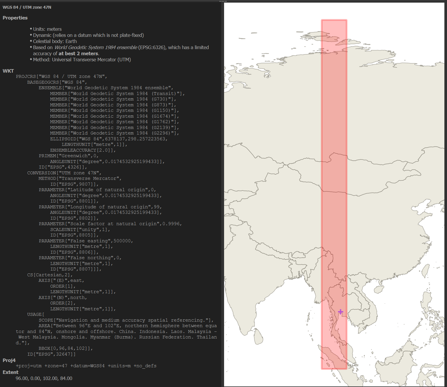
I've used EPSG:32647 for the map projection in this post. Below is QGIS' overview of this projection.
Maxar's Bangkok Satellite Imagery
I'll download one of Maxar's images of Bangkok along with its metadata.
$ wget -O ard_47_122022102202_2025-02-14_10400100A39C6A00-visual.tif \
    https://maxar-opendata.s3.amazonaws.com/events/Earthquake-Myanmar-March-2025/ard/47/122022102202/2025-02-14/10400100A39C6A00-visual.tif
$ wget https://raw.githubusercontent.com/opengeos/maxar-open-data/refs/heads/master/datasets/Earthquake-Myanmar-March-2025/10400100A39C6A00_union.geojson
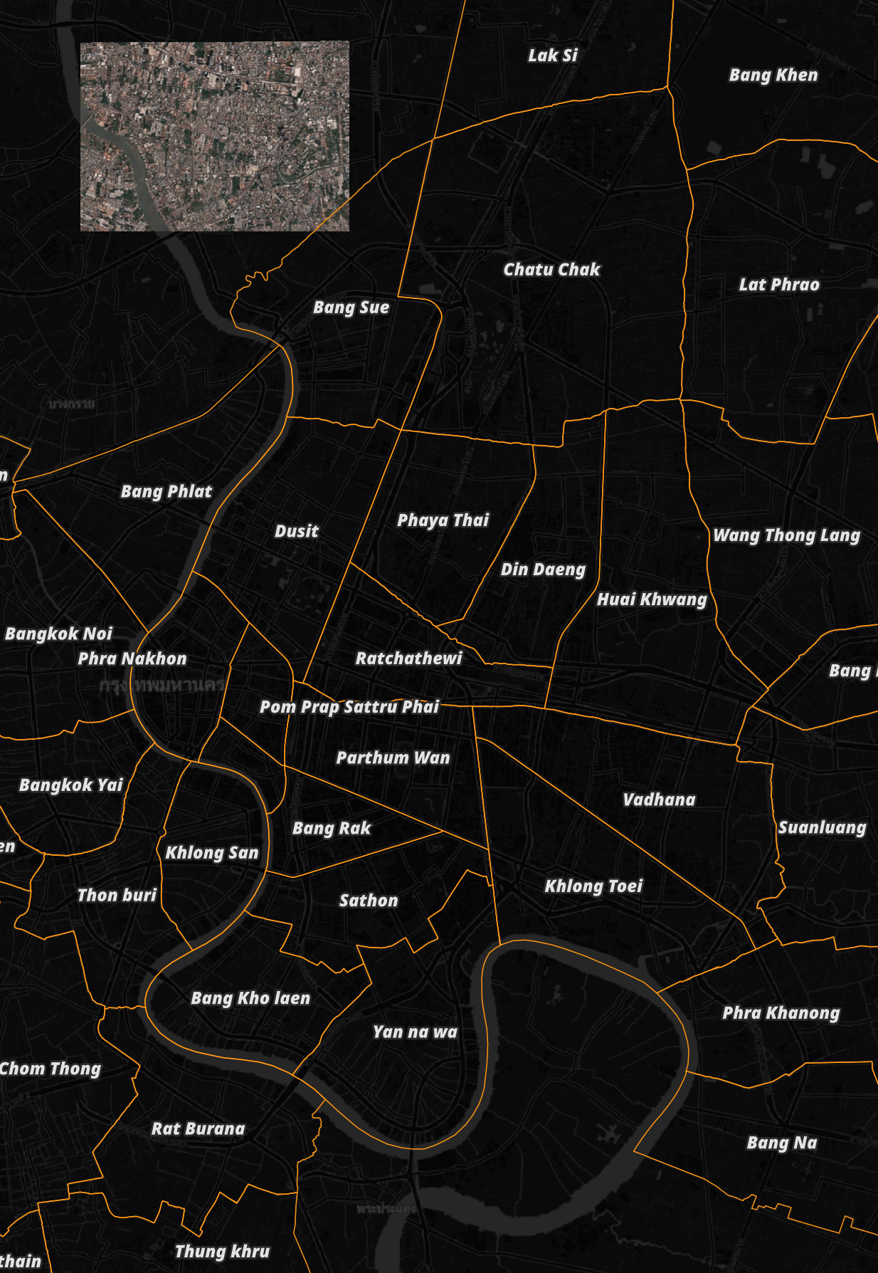
The image is a 17408 x 17408-pixel, 62 MB GeoTIFF. It has a 5.3 KM x 3.7 KM footprint and captures a area North West of Bangkok's Bang Sue district. Below is the image in relation to the rest of Bangkok.
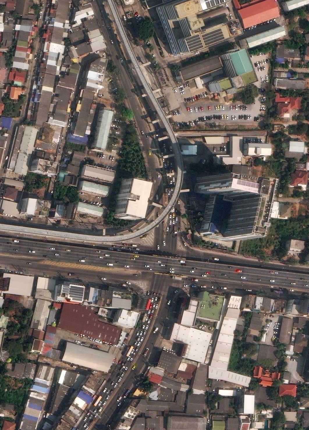
Below is a zoomed-in section of the image.
Below is the metadata for the image. It was taken on February 14th at 11:02AM local time. The image is free of any cloud cover.
$ jq -S .features[0].properties \
    10400100A39C6A00_union.geojson
{
  "ard_metadata_version": "0.0.1",
  "catalog_id": "10400100A39C6A00",
  "data-mask": "https://maxar-opendata.s3.amazonaws.com/events/Earthquake-Myanmar-March-2025/ard/47/122022102202/2025-02-14/10400100A39C6A00-data-mask.gpkg",
  "datetime": "2025-02-14T04:02:00Z",
  "grid:code": "MXRA-Z47-122022102202",
  "gsd": 0.35,
  "ms_analytic": "https://maxar-opendata.s3.amazonaws.com/events/Earthquake-Myanmar-March-2025/ard/47/122022102202/2025-02-14/10400100A39C6A00-ms.tif",
  "pan_analytic": "https://maxar-opendata.s3.amazonaws.com/events/Earthquake-Myanmar-March-2025/ard/47/122022102202/2025-02-14/10400100A39C6A00-pan.tif",
  "platform": "WV03",
  "proj:bbox": "659843.75,1529843.75,665156.25,1533587.620632182",
  "proj:code": "EPSG:32647",
  "proj:geometry": {
    "coordinates": [
      [
        [
          665156.25,
          1529843.75
        ],
        [
          659843.75,
          1529843.75
        ],
        [
          659843.75,
          1533553.3890408671
        ],
        [
          665156.25,
          1533587.6206321821
        ],
        [
          665156.25,
          1529843.75
        ]
      ]
    ],
    "type": "Polygon"
  },
  "quadkey": "122022102202",
  "tile:clouds_area": 0.0,
  "tile:clouds_percent": 0,
  "tile:data_area": 19.7,
  "utm_zone": 47,
  "view:azimuth": 262.1,
  "view:incidence_angle": 64.7,
  "view:off_nadir": 22.9,
  "view:sun_azimuth": 139.1,
  "view:sun_elevation": 55.2,
  "visual": "https://maxar-opendata.s3.amazonaws.com/events/Earthquake-Myanmar-March-2025/ard/47/122022102202/2025-02-14/10400100A39C6A00-visual.tif"
}
Detection Models
Below are the models that come packaged with GeoDeep. These are listed in geodeep/models.py. I've sorted this list for clarity.
MODELS = {
    'aerovision':   'aerovision16-yolo8.onnx',
    'birds':        'bird_detection_retinanet_deepforest.onnx',
    'buildings':    'buildings_ramp_XUnet_256.onnx',
    'cars':         'car_aerial_detection_yolo7_ITCVD_deepness.onnx',
    'planes':       'model_yolov7_tiny_planes_256.onnx',
    'roads':        'road_segmentation_model_with_metadata_26_10_22.onnx',
    'trees':        'tree_crown_detection_retinanet_deepforest.onnx',
    'trees_yolov9': 'yolov9_trees.onnx',
    'utilities':    'utilities-811-yolo8.onnx',
}
The first time you use these models, they'll be downloaded to ~/.cache/geodeep folder.
$ ls -lhS ~/.cache/geodeep
194M .. yolov9_trees.onnx
 94M .. road_segmentation_model_with_metadata_26_10_22.onnx
 79M .. buildings_ramp_XUnet_256.onnx
 32M .. tree_crown_detection_retinanet_deepforest.onnx
 24M .. car_aerial_detection_yolo7_ITCVD_deepness.onnx
 23M .. model_yolov7_tiny_planes_256.onnx
 11M .. aerovision16-yolo8.onnx
Models can be inspected with the following command.
$ geodeep-inspect cars
det_type: YOLO_v5_or_v7_default
det_conf: 0.3
det_iou_thresh: 0.8
classes: []
seg_thresh: 0.5
seg_small_segment: 11
resolution: 10.0
class_names: {'0': 'car'}
model_type: Detector
tiles_overlap: 10.0
tiles_size: 640
input_shape: [1, 3, 640, 640]
input_name: images
The following will show an overview of all the models.
$ python3
import json

from geodeep.inference import create_session
from geodeep           import models
from geodeep.models    import get_model_file


with open('models.json', 'w') as f:
    for model in models.list_models():
        _, config = create_session(get_model_file(model))
        config['model_name'] = model
        f.write(json.dumps(config, sort_keys=True) + '\n')
$ ~/duckdb
SELECT   * EXCLUDE(class_names),
         class_names::TEXT AS class_names
FROM     models.json
ORDER BY model_name;
┌─────────┬──────────┬────────────────┬──────────────────────┬────────────┬────────────────────┬──────────────┬────────────┬────────────┬───────────────────┬────────────┬───────────────┬────────────┬────────────────────────────────────────────────────┐
│ classes │ det_conf │ det_iou_thresh │       det_type       │ input_name │    input_shape     │  model_name  │ model_type │ resolution │ seg_small_segment │ seg_thresh │ tiles_overlap │ tiles_size │                    class_names                     │
│ json[]  │  double  │     double     │       varchar        │  varchar   │      int64[]       │   varchar    │  varchar   │   double   │       int64       │   double   │    double     │   int64    │                      varchar                       │
├─────────┼──────────┼────────────────┼──────────────────────┼────────────┼────────────────────┼──────────────┼────────────┼────────────┼───────────────────┼────────────┼───────────────┼────────────┼────────────────────────────────────────────────────┤
│ []      │      0.3 │            0.3 │ YOLO_v8              │ images     │ [1, 3, 640, 640]   │ aerovision   │ Detector   │       30.0 │                11 │        0.5 │          25.0 │        640 │ {'0': small-vehicle, '1': large-vehicle, '10': b…  │
│ []      │      0.4 │            0.4 │ retinanet            │ images     │ [1, 3, 1000, 1000] │ birds        │ Detector   │        2.0 │                11 │        0.5 │           5.0 │       1000 │ {'0': bird, '1': NULL, '10': NULL, '11': NULL, '…  │
│ []      │      0.3 │            0.8 │ YOLO_v5_or_v7_defa…  │ input      │ [1, 3, 256, 256]   │ buildings    │ Segmentor  │       50.0 │                11 │        0.5 │           5.0 │        256 │ {'0': Background, '1': Building, '10': NULL, '11…  │
│ []      │      0.3 │            0.8 │ YOLO_v5_or_v7_defa…  │ images     │ [1, 3, 640, 640]   │ cars         │ Detector   │       10.0 │                11 │        0.5 │          10.0 │        640 │ {'0': car, '1': NULL, '10': NULL, '11': NULL, '1…  │
│ []      │      0.3 │            0.3 │ YOLO_v5_or_v7_defa…  │ images     │ [1, 3, 256, 256]   │ planes       │ Detector   │       70.0 │                11 │        0.5 │           5.0 │        256 │ {'0': plane, '1': NULL, '10': NULL, '11': NULL, …  │
│ []      │      0.3 │            0.8 │ YOLO_v5_or_v7_defa…  │ input      │ [1, 3, 512, 512]   │ roads        │ Segmentor  │       21.0 │                11 │        0.5 │          15.0 │        512 │ {'0': not_road, '1': road, '10': NULL, '11': NUL…  │
│ []      │      0.3 │            0.4 │ retinanet            │ images     │ [1, 3, 400, 400]   │ trees        │ Detector   │       10.0 │                11 │        0.5 │           5.0 │        400 │ {'0': tree, '1': NULL, '10': NULL, '11': NULL, '…  │
│ []      │      0.5 │            0.4 │ YOLO_v9              │ images     │ [1, 3, 640, 640]   │ trees_yolov9 │ Detector   │       10.0 │                11 │        0.5 │          25.0 │        640 │ {'0': Tree, '1': NULL, '10': NULL, '11': NULL, '…  │
│ []      │      0.3 │            0.3 │ YOLO_v8              │ images     │ [1, 3, 640, 640]   │ utilities    │ Detector   │        3.0 │                11 │        0.5 │          10.0 │        640 │ {'0': Gas, '1':  Manhole, '10': NULL, '11': NULL…  │
└─────────┴──────────┴────────────────┴──────────────────────┴────────────┴────────────────────┴──────────────┴────────────┴────────────┴───────────────────┴────────────┴───────────────┴────────────┴────────────────────────────────────────────────────┘
GeoDeep's README on GitHub lists some details about the pre-built models as well as information on how you can create your own models using YOLO and at least 1,000 images.
Detecting Cars
The following car detection model only took a few moments to run on Maxar's image. It detected 304 cars.
$ geodeep \
    ard_47_122022102202_2025-02-14_10400100A39C6A00-visual.tif \
    cars \
    --output cars.geojson

$ jq -S '.features|length' cars.geojson # 304
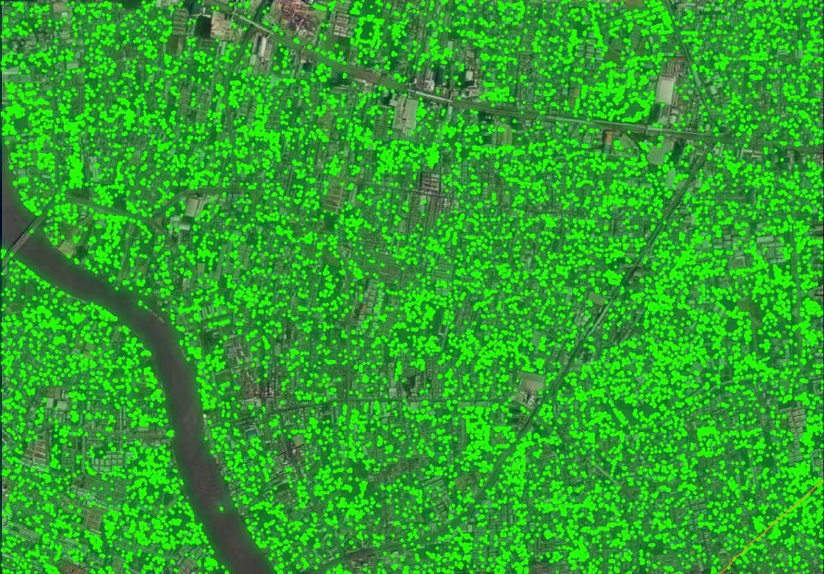
The following is an overview of where the detections were.
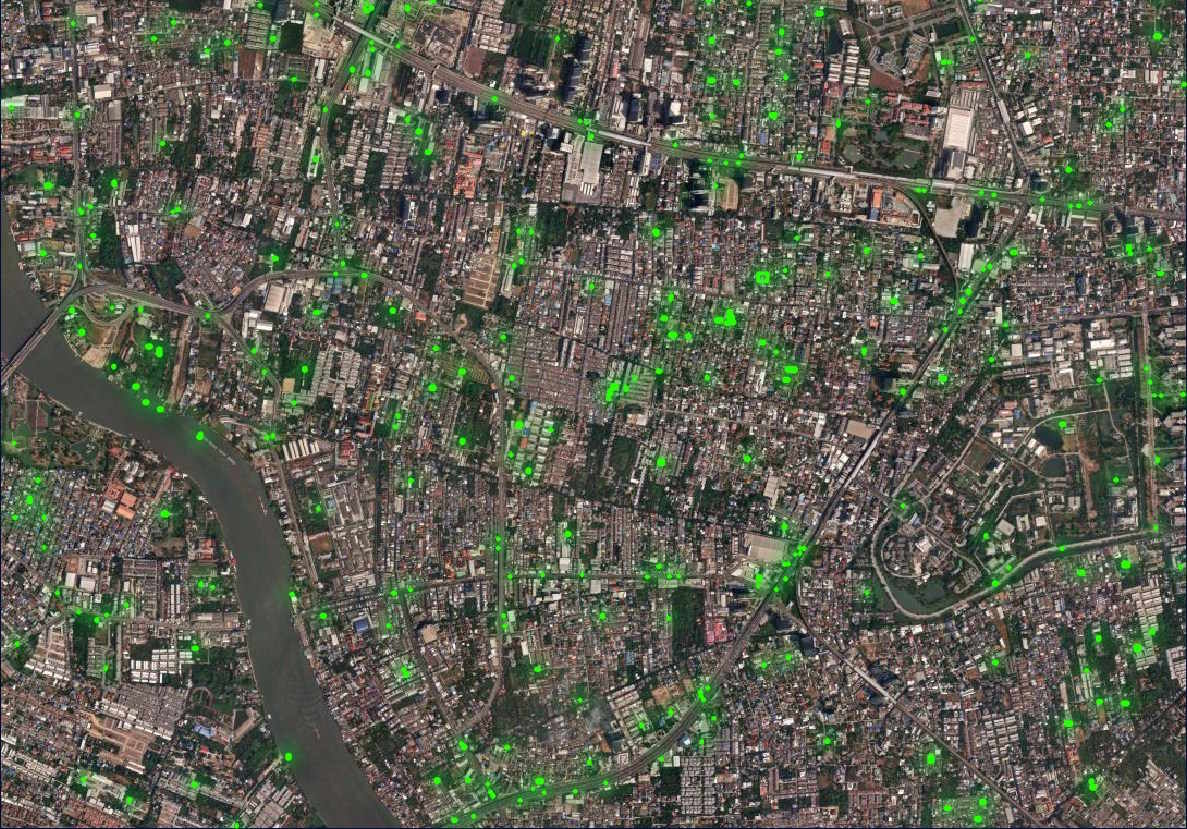
There were a large number of cars not detected by the model.
There were also a number of false-positives near the Chao Phraya River.
There was only a single detection class of "car" that appeared in the results. Below is the distribution of confidence scores.
$ jq '.features|.[]' \
     cars.geojson \
     > cars.unrolled.json
$ ~/duckdb
SELECT   ROUND(properties.score * 10)::int * 10 AS percent,
         COUNT(*) num_detections
FROM     READ_JSON('cars.unrolled.json')
GROUP BY 1
ORDER BY 1;
┌─────────┬────────────────┐
│ percent │ num_detections │
│  int32  │     int64      │
├─────────┼────────────────┤
│      30 │             86 │
│      40 │             97 │
│      50 │             50 │
│      60 │             34 │
│      70 │             25 │
│      80 │             10 │
│      90 │              2 │
└─────────┴────────────────┘
Detecting Trees
The tree detection model found 14,136 trees in Maxar's image.
$ geodeep \
    ard_47_122022102202_2025-02-14_10400100A39C6A00-visual.tif \
    trees \
    --output trees.geojson

$ jq -S '.features|length' trees.geojson # 14136
The model took a few minutes to run due to it running entirely on my CPU and not my GPU.
I couldn't see a flag to change the inference device to my Nvidia GPU in GeoDeep's codebase. I've raised an issue to see if GPU inference is in fact possible or could be supported.
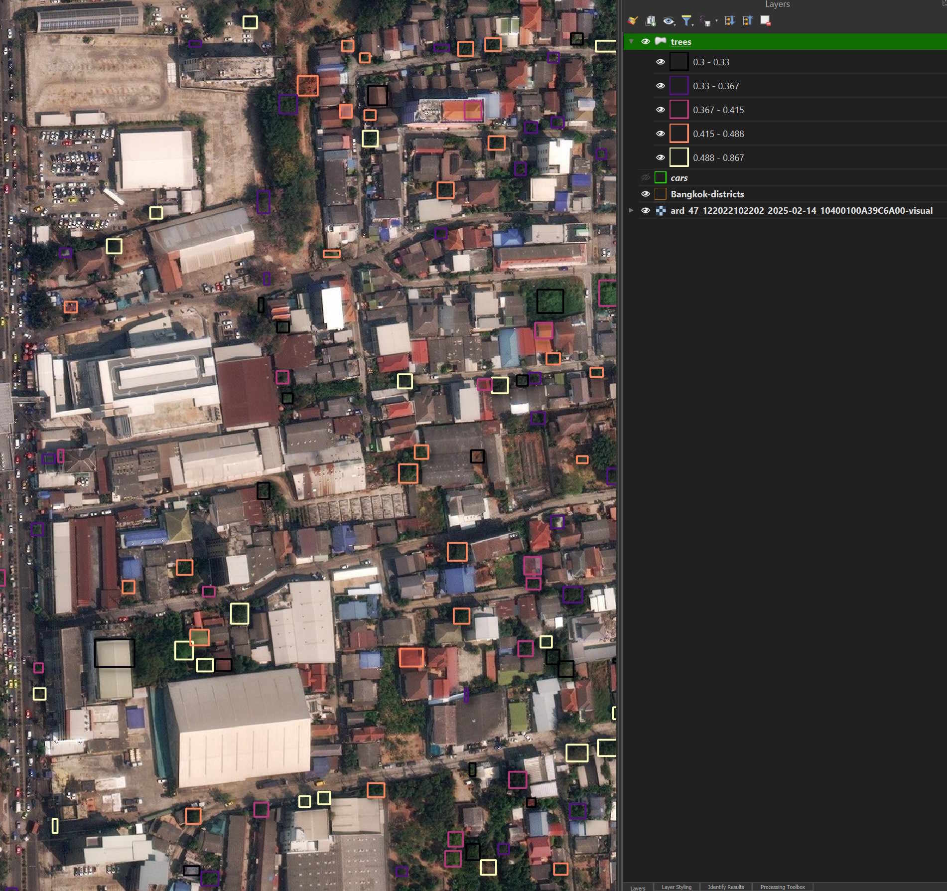
Here is an overview of the tree detections.
There are very few false-positives but a lot of trees are left undetected.
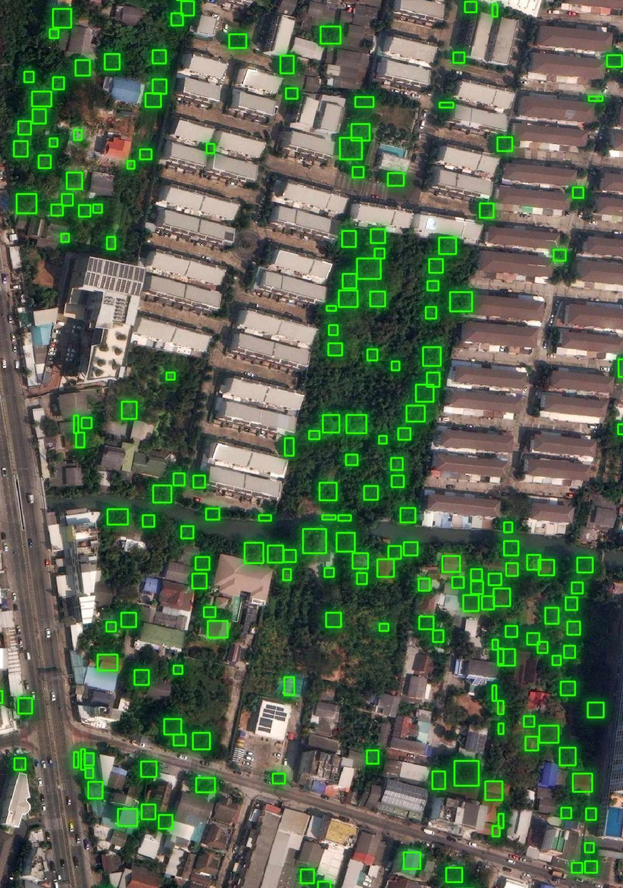
Few tree detections had a confidence value above 50% even though they're often spot-on.
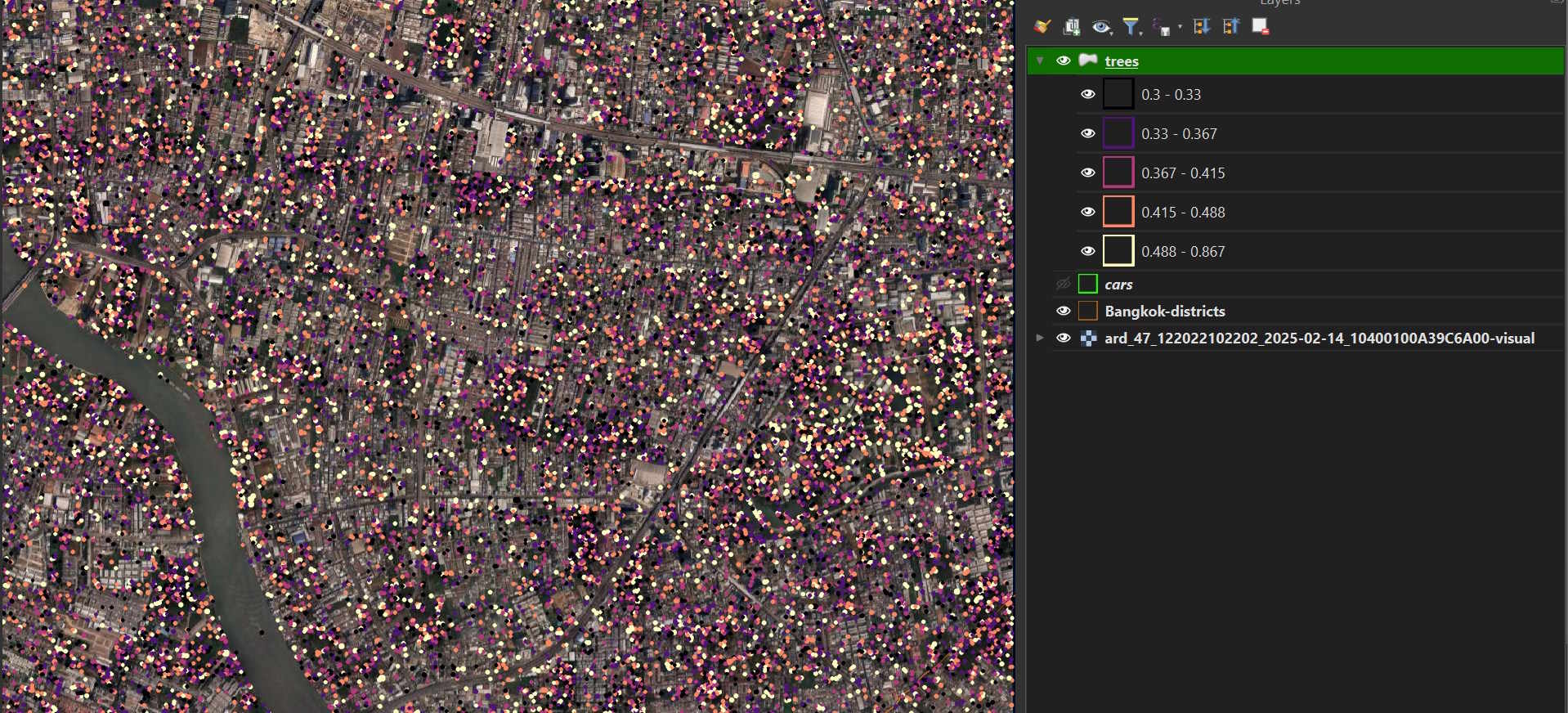
There was only a single detection class of "tree" that appeared in the results. Below is the distribution of confidence scores.
$ jq '.features|.[]' \
     trees.geojson \
     > trees.unrolled.json
$ ~/duckdb
SELECT   ROUND(properties.score * 10)::int * 10 AS percent,
         COUNT(*) num_detections
FROM     READ_JSON('trees.unrolled.json')
GROUP BY 1
ORDER BY 1;
┌─────────┬────────────────┐
│ percent │ num_detections │
│  int32  │     int64      │
├─────────┼────────────────┤
│      30 │           4412 │
│      40 │           5656 │
│      50 │           2678 │
│      60 │           1073 │
│      70 │            287 │
│      80 │             29 │
│      90 │              1 │
└─────────┴────────────────┘
Detecting Trees with YOLOv9
The following ran a lot faster than the previous model. It only took amount a minute to run. But with that said, only 402 trees were detected, two orders of magnitude less than the previous model.
$ geodeep \
    ard_47_122022102202_2025-02-14_10400100A39C6A00-visual.tif \
    trees_yolov9 \
    --output trees_yolov9.geojson

$ jq -S '.features|length' trees_yolov9.geojson # 402
There was only a single detection class of "Tree" that appeared in the results. Below is the distribution of confidence scores.
$ jq '.features|.[]' \
     trees_yolov9.geojson \
     > trees_yolov9.unrolled.json
$ ~/duckdb
SELECT   ROUND(properties.score * 10)::int * 10 AS percent,
         COUNT(*) num_detections
FROM     READ_JSON('trees_yolov9.unrolled.json')
GROUP BY 1
ORDER BY 1;
┌─────────┬────────────────┐
│ percent │ num_detections │
│  int32  │     int64      │
├─────────┼────────────────┤
│      50 │            106 │
│      60 │            187 │
│      70 │             92 │
│      80 │             15 │
│      90 │              2 │
└─────────┴────────────────┘
QGIS complained that the GeoJSON file was invalid so I converted it into a GPKG file.
$ ~/duckdb
COPY (
    SELECT ST_GEOMFROMGEOJSON(geometry) geom,
           ROUND(properties.score * 10)::int * 10 AS percent
    FROM   READ_JSON('trees_yolov9.unrolled.json',
                     maximum_object_size=100000000)
) TO 'trees_yolov9.gpkg'
        WITH (FORMAT GDAL,
              DRIVER 'GPKG',
              LAYER_CREATION_OPTIONS 'WRITE_BBOX=YES');
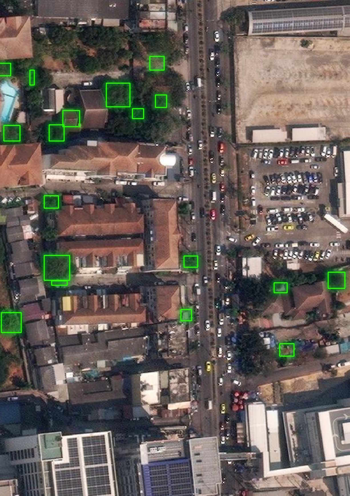
This is an overview of the detections.
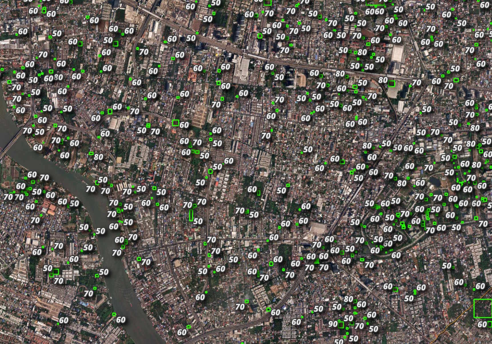
I didn't see many false-positives but lots of trees weren't detected.
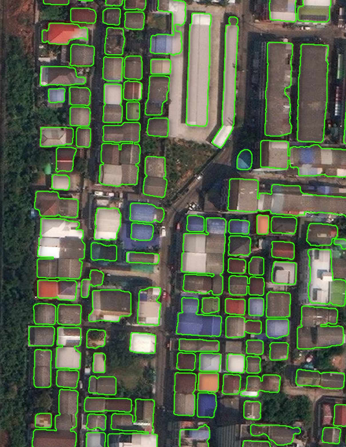
Detecting Buildings
The following model detected 23,561 buildings in Maxar's imagery.
$ geodeep \
    ard_47_122022102202_2025-02-14_10400100A39C6A00-visual.tif \
    buildings \
    --output buildings.geojson

$ jq -S '.features|length' buildings.geojson # 23561
This model doesn't report confidence values.
$  jq -S '.features[0]|del(.geometry)' \
         buildings.geojson
{
  "properties": {
    "class": "Building"
  },
  "type": "Feature"
}
The resulting GeoJSON file is 437 MB. When I tried to drag it into my QGIS project QGIS complained that it wasn't a valid data source. Below I converted the results into a 49 MB GeoPackage (GPKG) file.
There were 15 records classed as "Background" that I excluded from the GPKG file.
$ jq '.features|.[]' \
     buildings.geojson \
     > buildings.unrolled.json
$ ~/duckdb
COPY (
    SELECT ST_GEOMFROMGEOJSON(geometry) geom
    FROM   READ_JSON('buildings.unrolled.json',
                     maximum_object_size=100000000)
    WHERE  properties.class = 'Building'
) TO 'buildings.gpkg'
        WITH (FORMAT GDAL,
              DRIVER 'GPKG',
              LAYER_CREATION_OPTIONS 'WRITE_BBOX=YES');
Overview across the image.
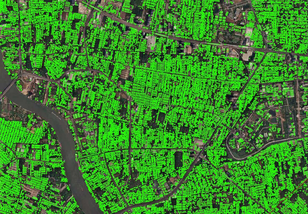
Some buildings are merged together but generally, anything that can be seen through the dense foliage is well-detected. A second-pass through an orthogonalising algorithm might help produce less wobbly outlines.
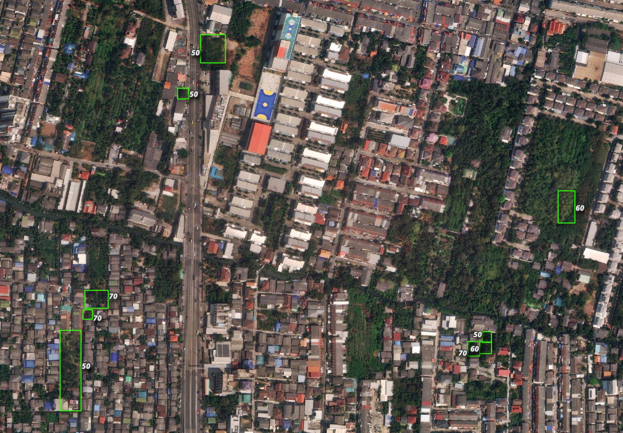
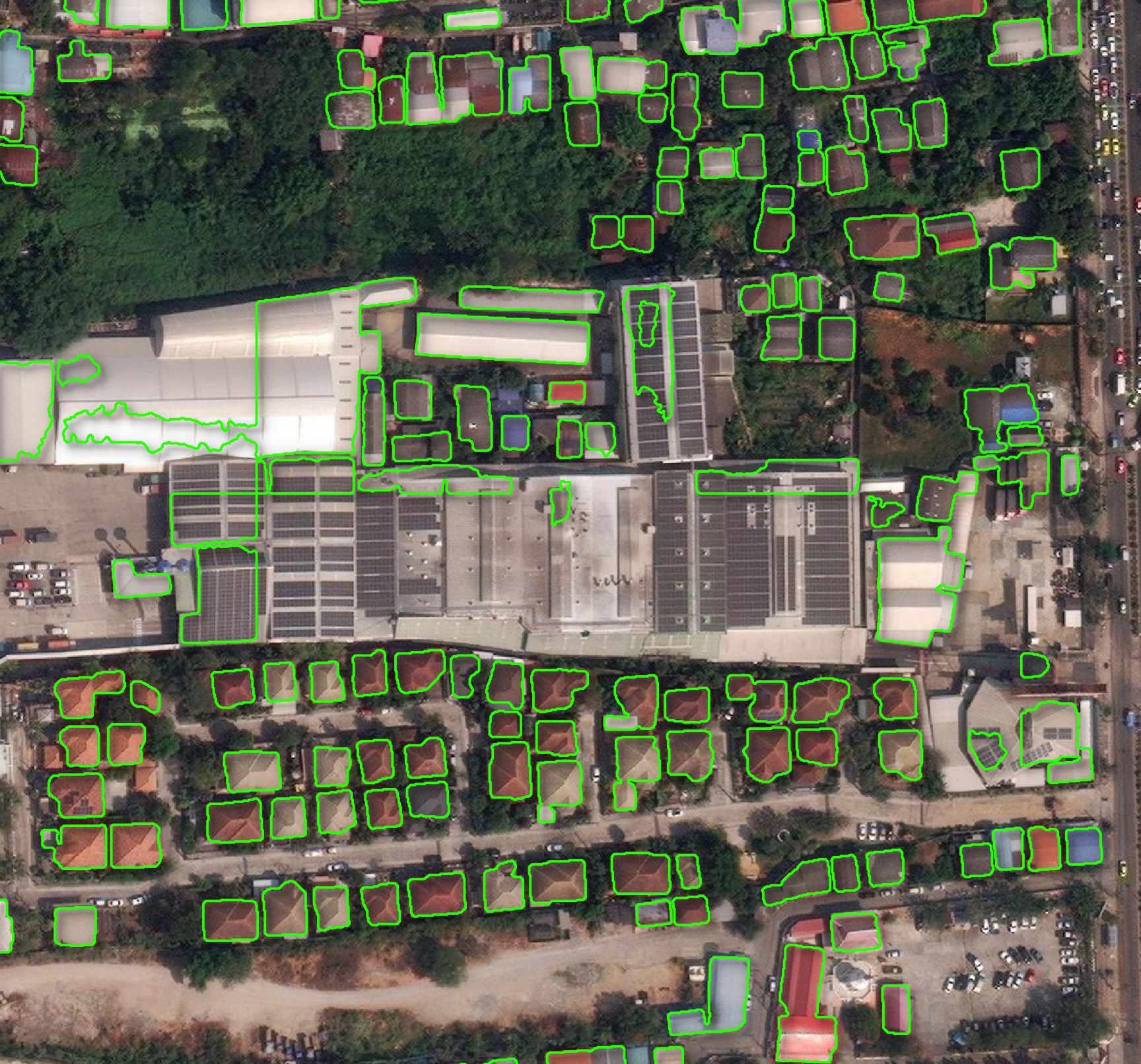
I did notice a large building wasn't picked out properly by the model.
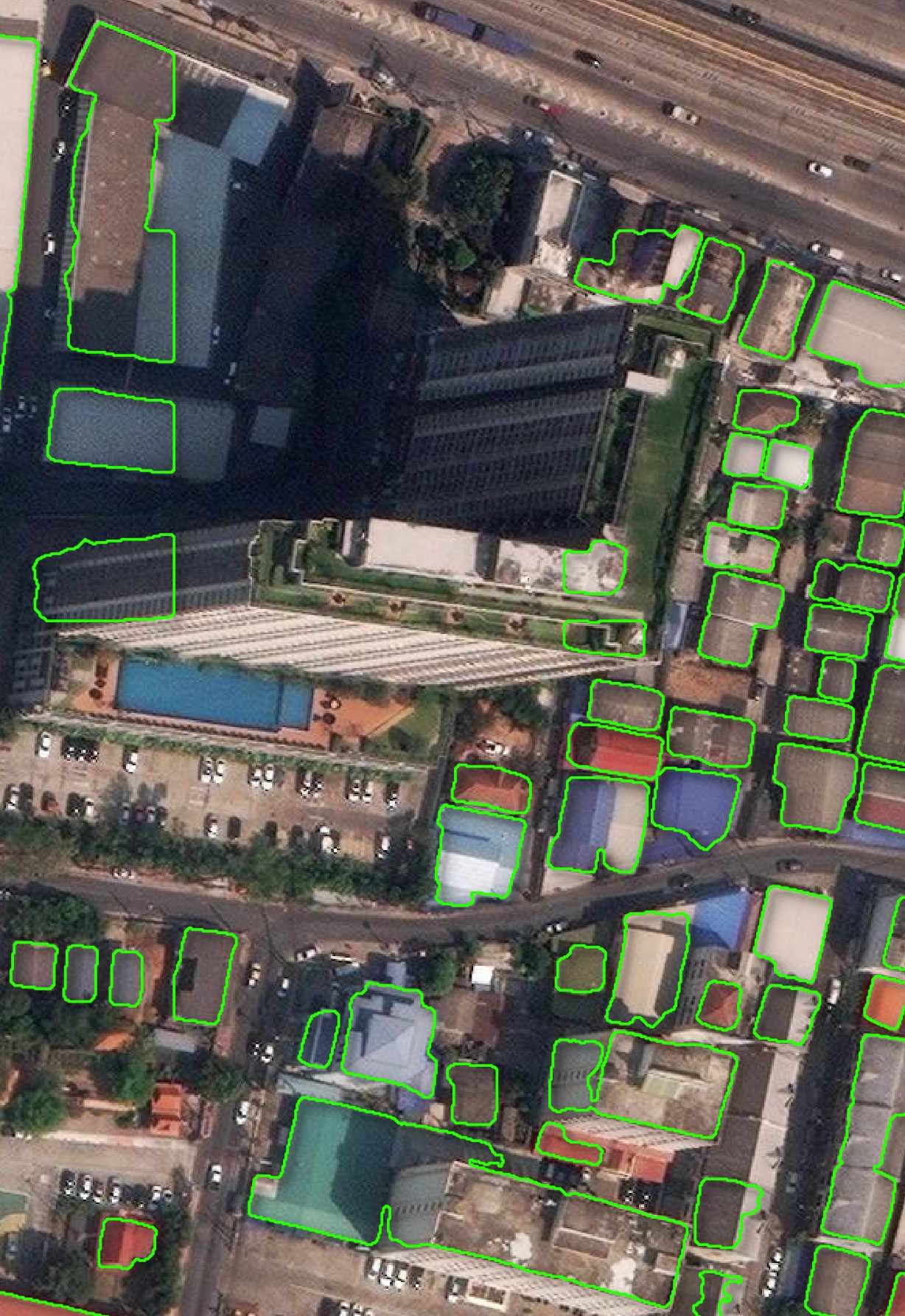
Below is another example of a large structure not being detected properly.
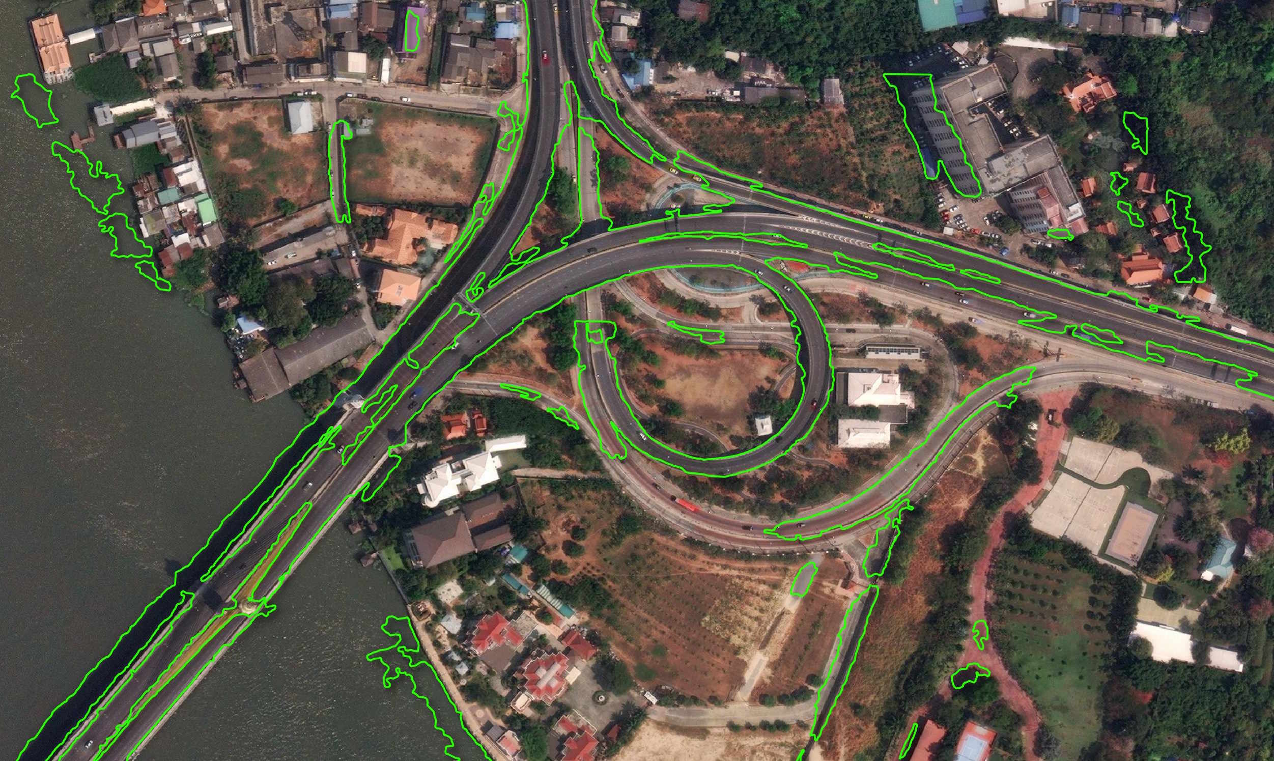
Detecting Roads
The following model detected 2,842 roads in the above image.
$ geodeep \
    ard_47_122022102202_2025-02-14_10400100A39C6A00-visual.tif \
    roads \
    --output roads.geojson
$ jq '.features|.[]' \
     roads.geojson \
     > roads.unrolled.json
$ ~/duckdb
There weren't any confidence scores reported but there are two classifications: "road" and "not_road."
SELECT   COUNT(*) num_detections,
         properties.class
FROM     READ_JSON('roads.unrolled.json',
                   maximum_object_size=1000000000)
GROUP BY 2;
┌────────────────┬──────────┐
│ num_detections │  class   │
│     int64      │ varchar  │
├────────────────┼──────────┤
│            136 │ not_road │
│           2842 │ road     │
└────────────────┴──────────┘
The resulting GeoJSON file is 181 MB and causes QGIS to slow down considerably. I'll convert it into a GPKG file so it renders faster.
$ ~/duckdb
COPY (
    SELECT ST_GEOMFROMGEOJSON(geometry) geom
    FROM   READ_JSON('roads.unrolled.json',
                     maximum_object_size=100000000)
    WHERE  properties.class = 'road'
) TO 'roads.gpkg'
  WITH (FORMAT GDAL,
        DRIVER 'GPKG',
        LAYER_CREATION_OPTIONS 'WRITE_BBOX=YES');
Below is an overview of the detected roads.
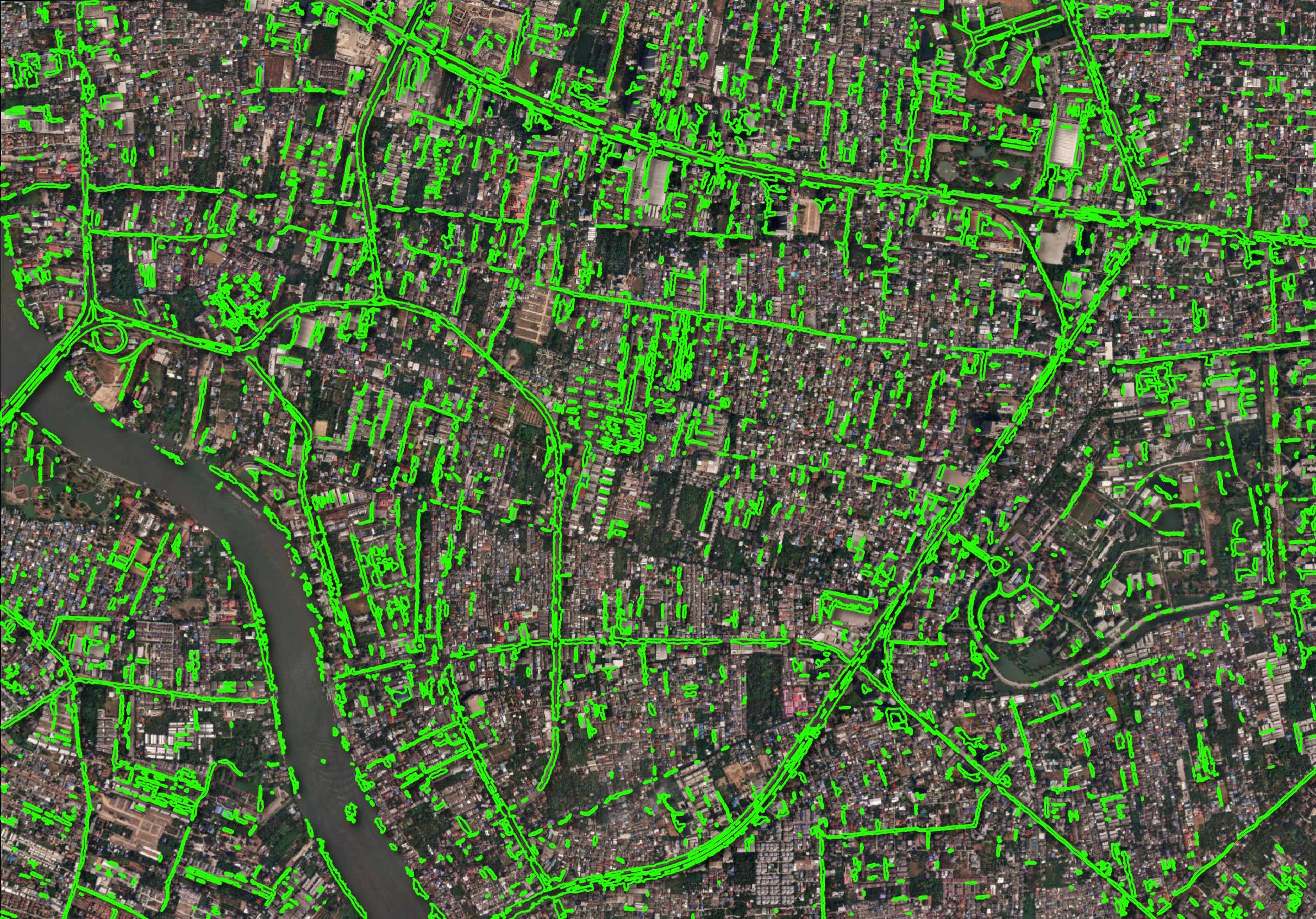
There are a lot of false-positives, incomplete detections and non-plausible outlines in the model's detections.
Detecting Planes
The Bangkok imagery from Maxar doesn't cover any of their airports. I'll download one of their images from Myanmar that has airports within its footprint.
$ wget -O ard_46_122000331100_2025-02-07_103001010E61BB00-visual.tif \
        https://maxar-opendata.s3.amazonaws.com/events/Earthquake-Myanmar-March-2025/ard/46/122000331100/2025-02-07/103001010E61BB00-visual.tif
Below is the metadata for the above image.
$ wget https://raw.githubusercontent.com/opengeos/maxar-open-data/refs/heads/master/datasets/Earthquake-Myanmar-March-2025/103001010E61BB00.geojson
$ jq -c .features[].properties 103001010E61BB00.geojson \
    | grep 122000331100 \
    | jq -S .
{
  "ard_metadata_version": "0.0.1",
  "catalog_id": "103001010E61BB00",
  "data-mask": "https://maxar-opendata.s3.amazonaws.com/events/Earthquake-Myanmar-March-2025/ard/46/122000331100/2025-02-07/103001010E61BB00-data-mask.gpkg",
  "datetime": "2025-02-07T04:01:56Z",
  "grid:code": "MXRA-Z46-122000331100",
  "gsd": 0.56,
  "ms_analytic": "https://maxar-opendata.s3.amazonaws.com/events/Earthquake-Myanmar-March-2025/ard/46/122000331100/2025-02-07/103001010E61BB00-ms.tif",
  "pan_analytic": "https://maxar-opendata.s3.amazonaws.com/events/Earthquake-Myanmar-March-2025/ard/46/122000331100/2025-02-07/103001010E61BB00-pan.tif",
  "platform": "WV02",
  "proj:bbox": "799843.75,2314843.75,805156.25,2318012.03454448",
  "proj:code": "EPSG:32646",
  "proj:geometry": {
    "coordinates": [
      [
        [
          805156.25,
          2314843.75
        ],
        [
          799843.75,
          2314843.75
        ],
        [
          799843.75,
          2317914.8673873823
        ],
        [
          805156.25,
          2318012.03454448
        ],
        [
          805156.25,
          2314843.75
        ]
      ]
    ],
    "type": "Polygon"
  },
  "quadkey": "122000331100",
  "tile:clouds_area": 0.0,
  "tile:clouds_percent": 0,
  "tile:data_area": 16.5,
  "utm_zone": 46,
  "view:azimuth": 135.0,
  "view:incidence_angle": 61.0,
  "view:off_nadir": 25.6,
  "view:sun_azimuth": 141.4,
  "view:sun_elevation": 45.2,
  "visual": "https://maxar-opendata.s3.amazonaws.com/events/Earthquake-Myanmar-March-2025/ard/46/122000331100/2025-02-07/103001010E61BB00-visual.tif"
}
The following model took less than a minute to run and detected 29 planes.
$ geodeep \
    ard_46_122000331100_2025-02-07_103001010E61BB00-visual.tif \
    planes \
    --output planes.geojson

$ jq -S '.features|length' planes.geojson # 29
$ jq '.features|.[]' \
     planes.geojson \
     > planes.unrolled.json
$ ~/duckdb
There is only a single detection class of "plane" in the results. Below are the distribution of confidence scores.
SELECT   ROUND(properties.score * 10)::int * 10 AS percent,
         COUNT(*) num_detections
FROM     READ_JSON('planes.unrolled.json')
GROUP BY 1
ORDER BY 1;
┌─────────┬────────────────┐
│ percent │ num_detections │
│  int32  │     int64      │
├─────────┼────────────────┤
│      30 │              9 │
│      40 │              8 │
│      50 │              4 │
│      60 │              1 │
│      70 │              3 │
│      80 │              3 │
│      90 │              1 │
└─────────┴────────────────┘
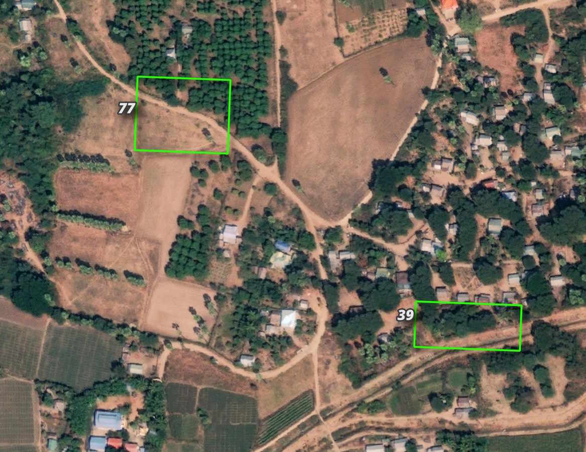
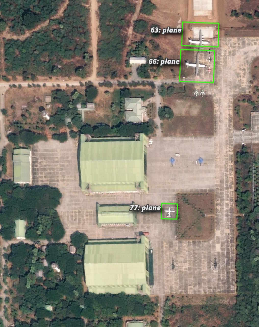
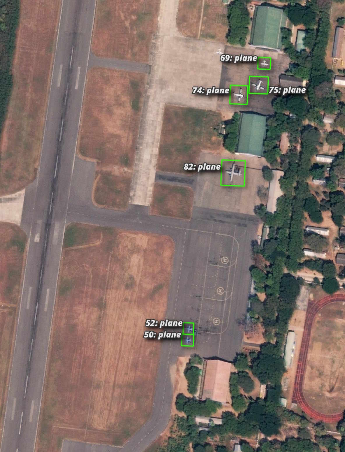
Most detections were false-positives but it did manage to detect most of the aircraft in the image. I've labelled the detections with their confidence value.
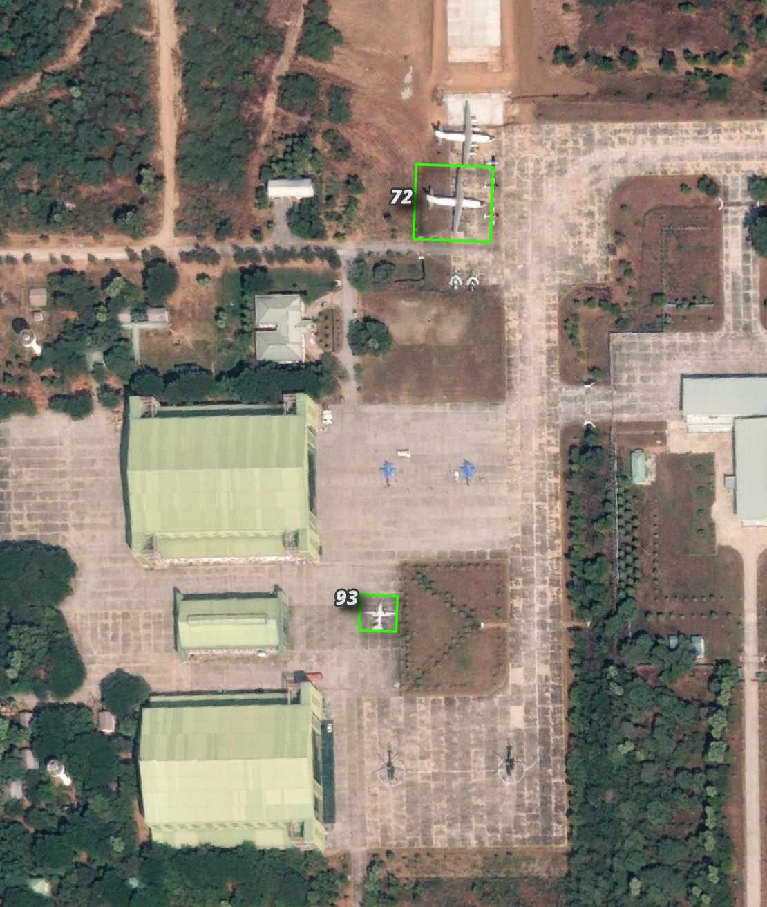
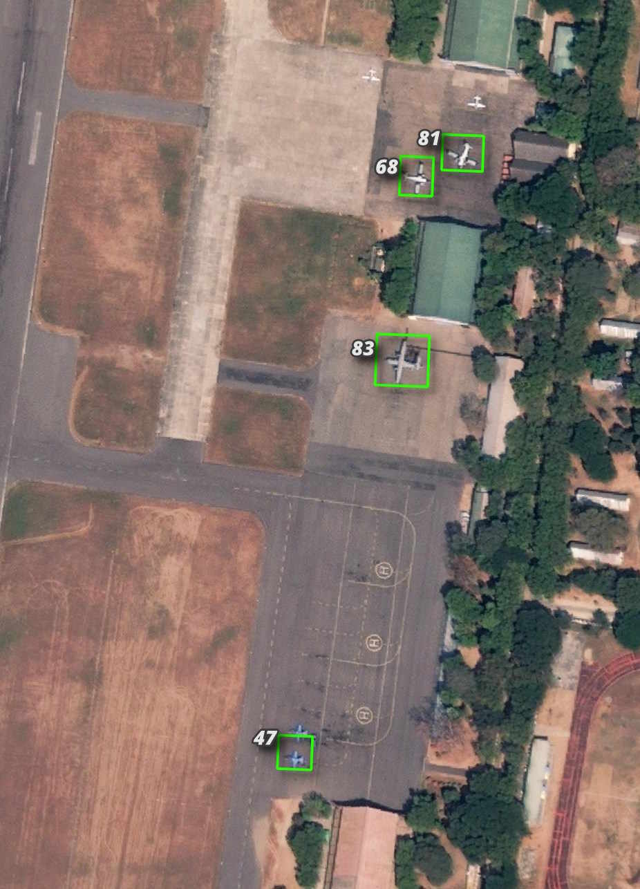
Some of the false-positives had pretty high confidence scores as well.
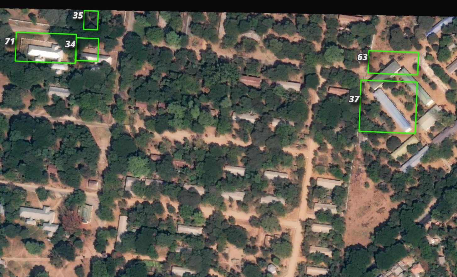
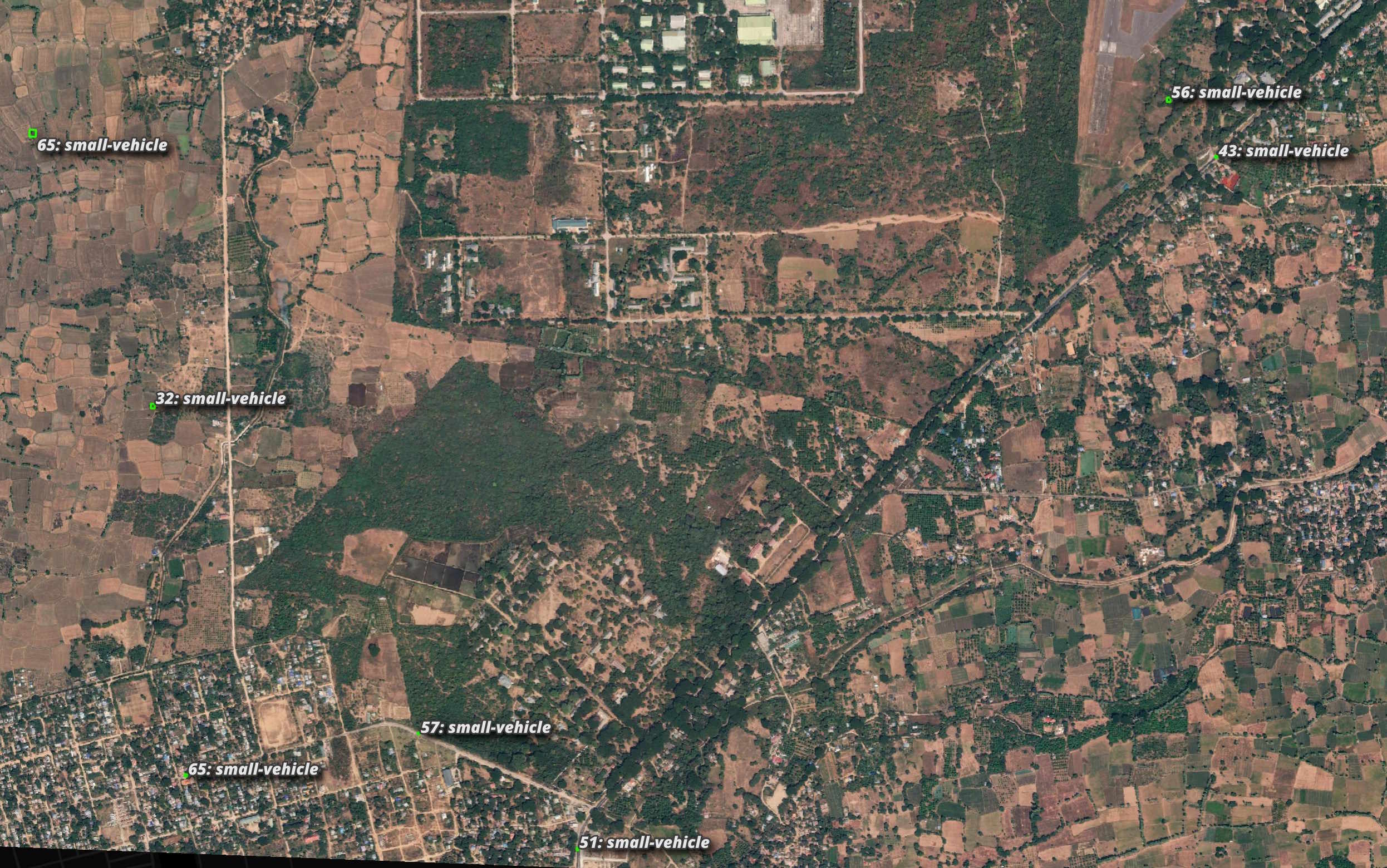
Multi-Class Object Detection
The following model took less than a minute to run and detected 44 features.
$ geodeep \
    ard_46_122000331100_2025-02-07_103001010E61BB00-visual.tif \
    aerovision \
    --output aerovision.geojson

$ jq -S '.features|length' aerovision.geojson # 44
Below is a breakdown of detections by classification and confidence value.
$ jq '.features|.[]' \
     aerovision.geojson \
     > aerovision.unrolled.json
$ ~/duckdb
WITH a AS (
    SELECT   ROUND(properties.score * 10)::int * 10 AS percent,
             properties.class AS classification,
             COUNT(*) num_detections
    FROM     READ_JSON('aerovision.unrolled.json')
    GROUP BY 1, 2
)
PIVOT    a
ON       percent
USING    SUM(num_detections)
GROUP BY classification;
┌────────────────┬────────┬────────┬────────┬────────┬────────┬────────┬────────┐
│ classification │   30   │   40   │   50   │   60   │   70   │   80   │   90   │
│    varchar     │ int128 │ int128 │ int128 │ int128 │ int128 │ int128 │ int128 │
├────────────────┼────────┼────────┼────────┼────────┼────────┼────────┼────────┤
│ small-vehicle  │      1 │      1 │      1 │      4 │        │        │        │
│ baseball-field │      1 │      1 │      1 │      3 │        │        │        │
│ road-circle    │        │        │        │      1 │        │        │        │
│ large-vehicle  │      3 │      1 │        │        │        │        │        │
│ swimming-pool  │        │      3 │      7 │      2 │      1 │      1 │      1 │
│ plane          │        │        │      2 │      1 │      4 │      2 │        │
│ tennis-court   │        │      1 │        │      1 │        │        │        │
└────────────────┴────────┴────────┴────────┴────────┴────────┴────────┴────────┘
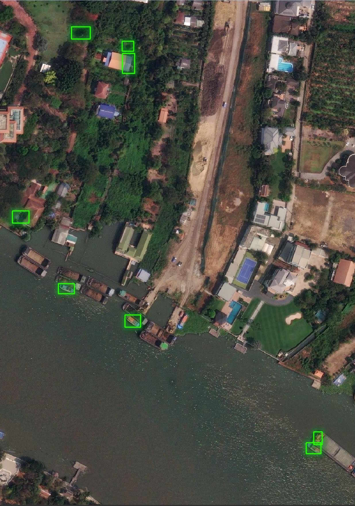
The plane detection was pretty good.
All of the "large-vehicle" detections were buildings. I couldn't see any baseball fields, swimming polls or tennis courts in Maxar's image so I'll have to call all those detections false-positives.
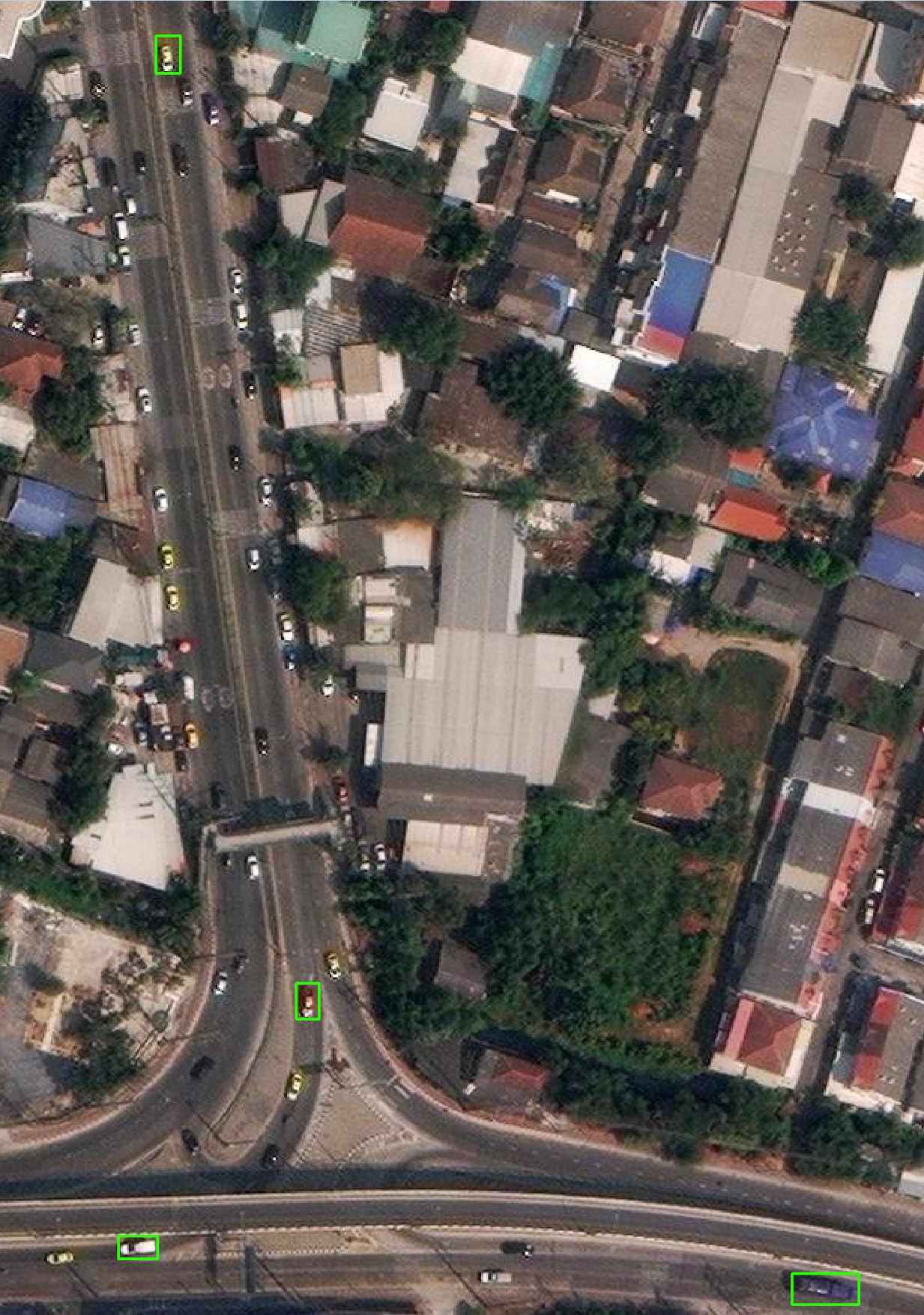
Half of the "small-vehicle" detections were spot on. Below is a screen shot of them.