France runs a public data platform with 74K datasets and APIs containing and/or representing 387K files from 6K organisations. "My Mobile Network" is a group of datasets hosted on this platform. It contains six datasets describing the structure and performance of France's mobile networks.
These datasets include the locations, operators and capabilities of mobile sites, theoretical coverage of these networks, performance measurements against popular websites and several other metrics.
In this post, I'll walk through converting a few of these datasets into Parquet and examining their features.
My Workstation
I'm using a 5.7 GHz AMD Ryzen 9 9950X CPU. It has 16 cores and 32 threads and 1.2 MB of L1, 16 MB of L2 and 64 MB of L3 cache. It has a liquid cooler attached and is housed in a spacious, full-sized Cooler Master HAF 700 computer case.
The system has 96 GB of DDR5 RAM clocked at 4,800 MT/s and a 5th-generation, Crucial T700 4 TB NVMe M.2 SSD which can read at speeds up to 12,400 MB/s. There is a heatsink on the SSD to help keep its temperature down. This is my system's C drive.
The system is powered by a 1,200-watt, fully modular Corsair Power Supply and is sat on an ASRock X870E Nova 90 Motherboard.
I'm running Ubuntu 24 LTS via Microsoft's Ubuntu for Windows on Windows 11 Pro. In case you're wondering why I don't run a Linux-based desktop as my primary work environment, I'm still using an Nvidia GTX 1080 GPU which has better driver support on Windows and ArcGIS Pro only supports Windows natively.
Installing Prerequisites
I'll use GDAL 3.9.3, Python 3.12.3 and a few other tools to help analyse the data in this post.
$ sudo add-apt-repository ppa:deadsnakes/ppa
$ sudo add-apt-repository ppa:ubuntugis/ubuntugis-unstable
$ sudo apt update
$ sudo apt install \
    gdal-bin \
    jq \
    python3-pip \
    python3.12-venv
Below, I'll set up a Python Virtual Environment and install some dependencies.
$ python3 -m venv ~/.france-mobile
$ source ~/.france-mobile/bin/activate
$ python3 -m pip install \
    duckdb \
    py7zr \
    rich \
    shpyx
I'll use DuckDB, along with its H3, JSON, Lindel, Parquet and Spatial extensions in this post.
$ cd ~
$ wget -c https://github.com/duckdb/duckdb/releases/download/v1.5.1/duckdb_cli-linux-amd64.zip
$ unzip -j duckdb_cli-linux-amd64.zip
$ chmod +x duckdb
$ ~/duckdb
INSTALL h3 FROM community;
INSTALL lindel FROM community;
INSTALL json;
INSTALL parquet;
INSTALL spatial;
I'll set up DuckDB to load every installed extension each time it launches.
$ vi ~/.duckdbrc
.timer on
.width 180
LOAD h3;
LOAD lindel;
LOAD json;
LOAD parquet;
LOAD spatial;
The maps in this post were rendered with QGIS version 4.0.0. QGIS is a desktop application that runs on Windows, macOS and Linux. The application has grown in popularity in recent years and has ~15M application launches from users all around the world each month.
I used QGIS' HCMGIS plugin to add basemaps from Esri to this post.
Metropolitan, Overseas & Departments of France
Metropolitan and Overseas France will be mentioned a lot in these datasets and files are often partitioned by these geographies.
Below is Metropolitan France, the hexagon-shaped landmass found in Europe.
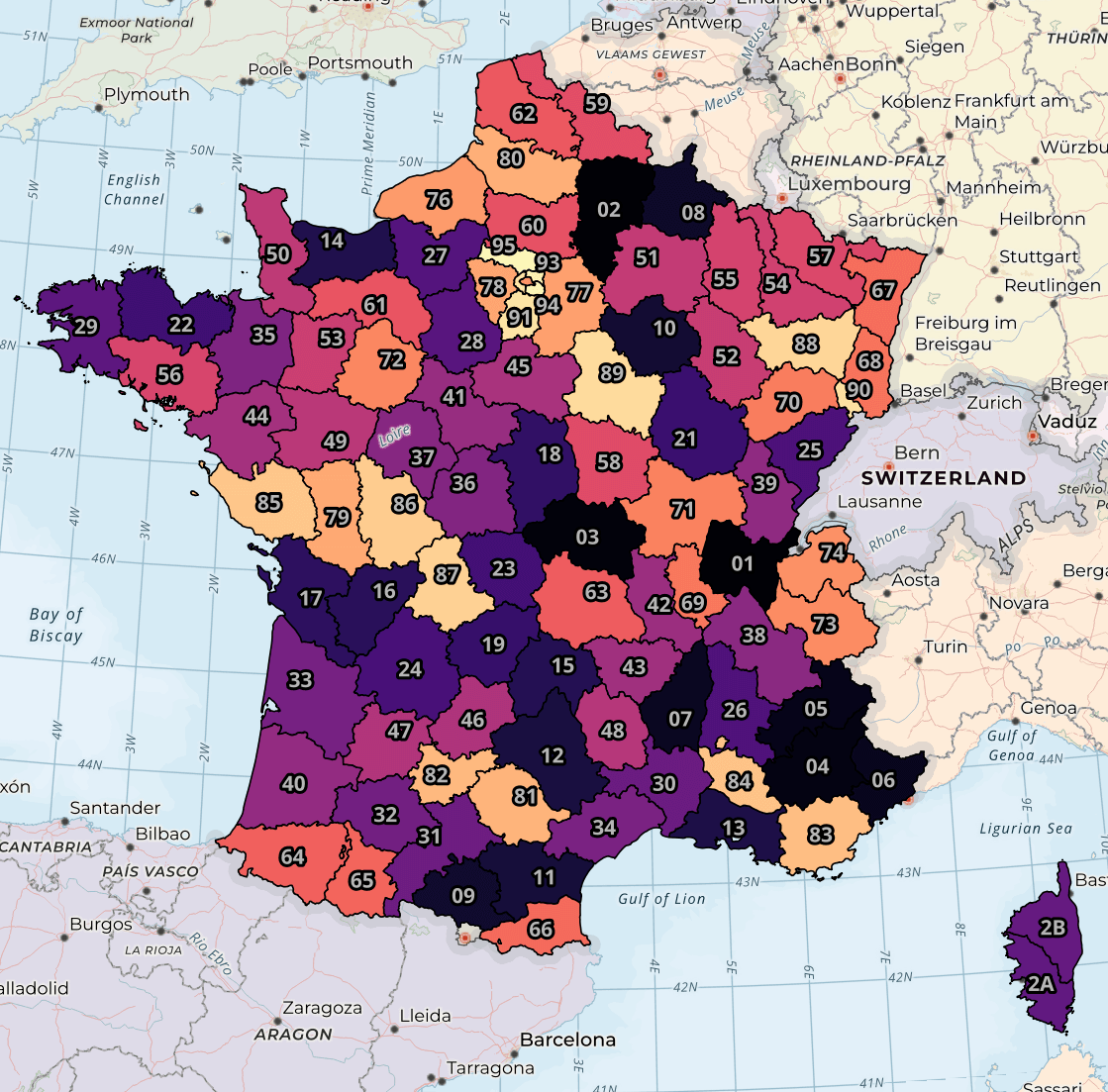
I've coloured each department above by its number with the brightest colours being the highest values. The polygons and their labels were sourced from this gist. There isn't a strong geographic relationship between a department number and its location.
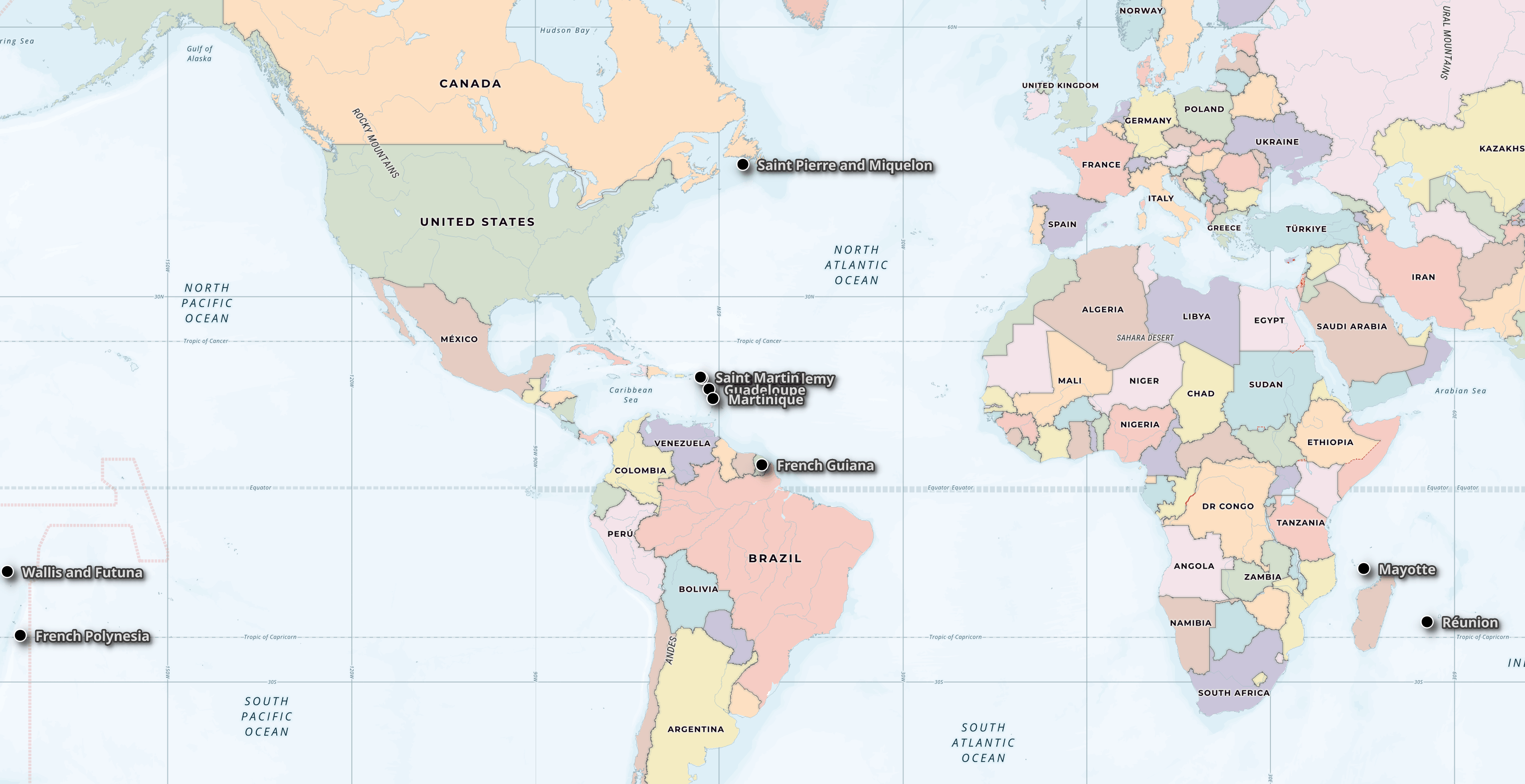
Below are ten of the eleven inhabited French overseas territories. Apologies for Saint Barthélemy's label being obscured by Saint Martin's.
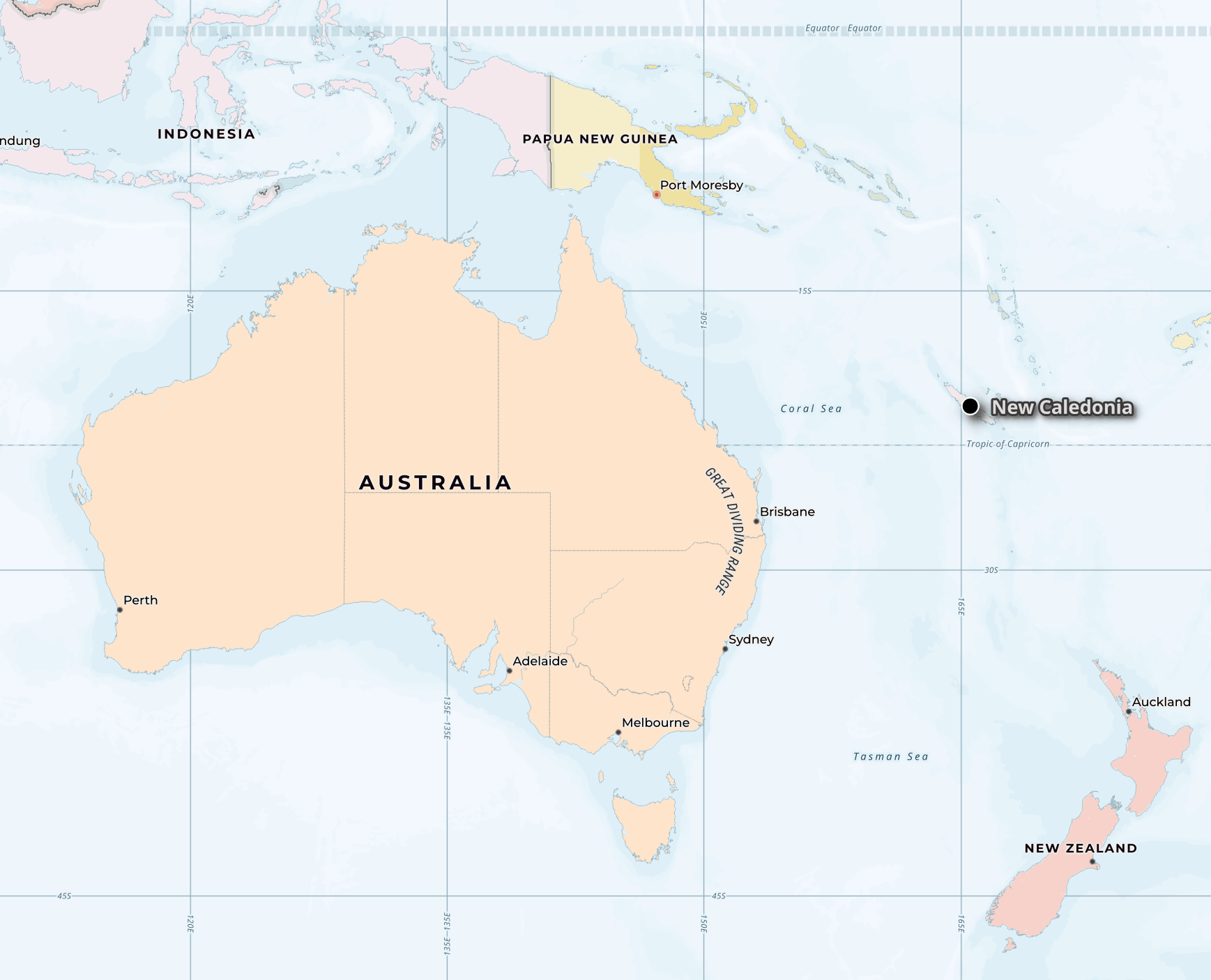
Below is the 11th, New Caledonia, with its proximity to Australia and New Zealand.
Mobile Service Sites
The "Mobile Service Sites" dataset contains every French mobile provider's cell sites' capabilities for every quarter going back to 2017. Below, I've downloaded the latest quarter's CSV file. I'll import it into DuckDB.
$ ~/duckdb
CREATE OR REPLACE TABLE a AS
    FROM READ_CSV('2025_T4_sites_Metropole.csv',
                  decimal_separator=',');
The CSV file contains 123K rows.
SELECT COUNT(*) FROM a; -- 123068
These are the unique value counts and NULL % for each of the columns. The dataset contains the date when 5G was first activated at any site that supports it, several columns describing the geography and each site's network generation support.
SELECT   column_name,
         column_type[:30],
         null_percentage,
         approx_unique,
         min[:30],
         max[:30]
FROM     (SUMMARIZE
          FROM a)
ORDER BY LOWER(column_name);
┌──────────────────────────────┬──────────────────────────┬─────────────────┬───────────────┬─────────────────────────────┬────────────────────────┐
│         column_name          │     column_type[:30]     │ null_percentage │ approx_unique │          min[:30]           │        max[:30]        │
│           varchar            │         varchar          │  decimal(9,2)   │     int64     │           varchar           │        varchar         │
├──────────────────────────────┼──────────────────────────┼─────────────────┼───────────────┼─────────────────────────────┼────────────────────────┤
│ code_op                      │ BIGINT                   │            0.00 │             3 │ 20801                       │ 20820                  │
│ date_ouverturecommerciale_5g │ TIMESTAMP WITH TIME ZONE │           41.42 │          1636 │ 2020-10-09 03:00:00+03      │ 2025-12-31 02:00:00+02 │
│ id_site_partage              │ VARCHAR                  │           78.48 │          5065 │ 2019_LOT1_Site_ZG_03_003_S5 │ ZPZ95405               │
│ id_station_anfr              │ VARCHAR                  │            0.47 │         89043 │ 00008962D1                  │ 0952750744             │
│ insee_com                    │ VARCHAR                  │            0.00 │         20391 │ 01001                       │ 95690                  │
│ insee_dep                    │ VARCHAR                  │            0.00 │            90 │ 01                          │ 95                     │
│ latitude                     │ DOUBLE                   │            0.00 │         69205 │ 41.36445                    │ 51.08034               │
│ longitude                    │ DOUBLE                   │            0.00 │         66599 │ -5.08888                    │ 9.55028                │
│ mes_4g_trim                  │ BIGINT                   │            0.00 │             2 │ 0                           │ 1                      │
│ nom_com                      │ VARCHAR                  │            0.00 │         25727 │ Aast                        │ Œuilly                 │
│ nom_dep                      │ VARCHAR                  │            0.00 │            89 │ Ain                         │ Yvelines               │
│ nom_op                       │ VARCHAR                  │            0.00 │             4 │ Bouygues Telecom            │ SFR                    │
│ nom_reg                      │ VARCHAR                  │            0.00 │            15 │ Auvergne-Rhône-Alpes        │ Île-de-France          │
│ num_site                     │ VARCHAR                  │            0.00 │        128897 │ 00000001A1                  │ TA0005                 │
│ site_2g                      │ BIGINT                   │            0.00 │             2 │ 0                           │ 1                      │
│ site_3g                      │ BIGINT                   │            0.00 │             2 │ 0                           │ 1                      │
│ site_4g                      │ BIGINT                   │            0.00 │             2 │ 0                           │ 1                      │
│ site_5g                      │ BIGINT                   │            0.00 │             2 │ 0                           │ 1                      │
│ site_5g_1800_m_hz            │ BIGINT                   │            0.00 │             1 │ 0                           │ 0                      │
│ site_5g_2100_m_hz            │ BIGINT                   │            0.00 │             2 │ 0                           │ 1                      │
│ site_5g_3500_m_hz            │ BIGINT                   │            0.00 │             2 │ 0                           │ 1                      │
│ site_5g_700_m_hz             │ BIGINT                   │            0.00 │             2 │ 0                           │ 1                      │
│ site_5g_800_m_hz             │ BIGINT                   │            0.00 │             1 │ 0                           │ 0                      │
│ site_capa_240mbps            │ BIGINT                   │            0.00 │             2 │ 0                           │ 1                      │
│ site_DCC                     │ BIGINT                   │            0.00 │             2 │ 0                           │ 1                      │
│ site_strategique             │ BIGINT                   │            0.00 │             2 │ 0                           │ 1                      │
│ site_ZB                      │ BIGINT                   │            0.00 │             2 │ 0                           │ 1                      │
│ x                            │ DOUBLE                   │            0.00 │         83320 │ 102979.0                    │ 1240681.0              │
│ y                            │ DOUBLE                   │            0.00 │         92010 │ 6050020.0                   │ 7109525.0              │
└──────────────────────────────┴──────────────────────────┴─────────────────┴───────────────┴─────────────────────────────┴────────────────────────┘
Below are the number of sites for each network operator. Note, this file is only for Metropolitan France, not its overseas territories.
SELECT   COUNT(*),
         nom_op
FROM     a
GROUP BY 2
ORDER BY 1 DESC;
┌──────────────┬──────────────────┐
│ count_star() │      nom_op      │
│    int64     │     varchar      │
├──────────────┼──────────────────┤
│        32367 │ Orange           │
│        30286 │ Free Mobile      │
│        30255 │ Bouygues Telecom │
│        30160 │ SFR              │
└──────────────┴──────────────────┘
Below is the number of sites supporting each network generation broken down by operator.
SELECT   nom_op,
         "2g":          COUNT(*) FILTER(site_2g),
         "3g":          COUNT(*) FILTER(site_3g),
         "4g":          COUNT(*) FILTER(site_4g),
         "5g":          COUNT(*) FILTER(site_5g),
         "5g_1800":     COUNT(*) FILTER(site_5g_1800_m_hz),
         "5g_2100":     COUNT(*) FILTER(site_5g_2100_m_hz),
         "5g_3500":     COUNT(*) FILTER(site_5g_3500_m_hz),
         "5g_700":      COUNT(*) FILTER(site_5g_700_m_hz),
         "5g_800":      COUNT(*) FILTER(site_5g_800_m_hz),
         "capa_240":    COUNT(*) FILTER(site_capa_240mbps),
         "DCC":         COUNT(*) FILTER(site_DCC),
         "strategique": COUNT(*) FILTER(site_strategique),
         "ZB":          COUNT(*) FILTER(site_ZB)
FROM     a
GROUP BY 1;
┌──────────────────┬───────┬───────┬───────┬───────┬─────────┬─────────┬─────────┬────────┬────────┬──────────┬───────┬─────────────┬───────┐
│      nom_op      │  2g   │  3g   │  4g   │  5g   │ 5g_1800 │ 5g_2100 │ 5g_3500 │ 5g_700 │ 5g_800 │ capa_240 │  DCC  │ strategique │  ZB   │
│     varchar      │ int64 │ int64 │ int64 │ int64 │  int64  │  int64  │  int64  │ int64  │ int64  │  int64   │ int64 │    int64    │ int64 │
├──────────────────┼───────┼───────┼───────┼───────┼─────────┼─────────┼─────────┼────────┼────────┼──────────┼───────┼─────────────┼───────┤
│ SFR              │ 21990 │ 29199 │ 30144 │ 16089 │       0 │   11578 │   10507 │      0 │      0 │    27983 │  3925 │          36 │  2647 │
│ Bouygues Telecom │ 19556 │ 28590 │ 30222 │ 17636 │       0 │   17377 │   10513 │      0 │      0 │    27838 │  3929 │          36 │  2647 │
│ Orange           │ 15531 │ 29649 │ 32327 │ 15875 │       0 │    2232 │   13508 │  12548 │      0 │    31123 │  3936 │          36 │  2648 │
│ Free Mobile      │     0 │  6654 │ 30266 │ 22499 │       0 │       0 │   10501 │  21080 │      0 │    30130 │  3961 │          36 │  2647 │
└──────────────────┴───────┴───────┴───────┴───────┴─────────┴─────────┴─────────┴────────┴────────┴──────────┴───────┴─────────────┴───────┘
I'll export this table to a Parquet file.
COPY (
    SELECT   * EXCLUDE(latitude, longitude),
             geometry: ST_POINT(longitude, latitude)
    FROM     a
    ORDER BY HILBERT_ENCODE([latitude,
                             longitude]::double[2])
) TO '2025_T4_sites_Metropole.parquet' (
        FORMAT 'PARQUET',
        CODEC  'ZSTD',
        COMPRESSION_LEVEL 22,
        ROW_GROUP_SIZE 15000);
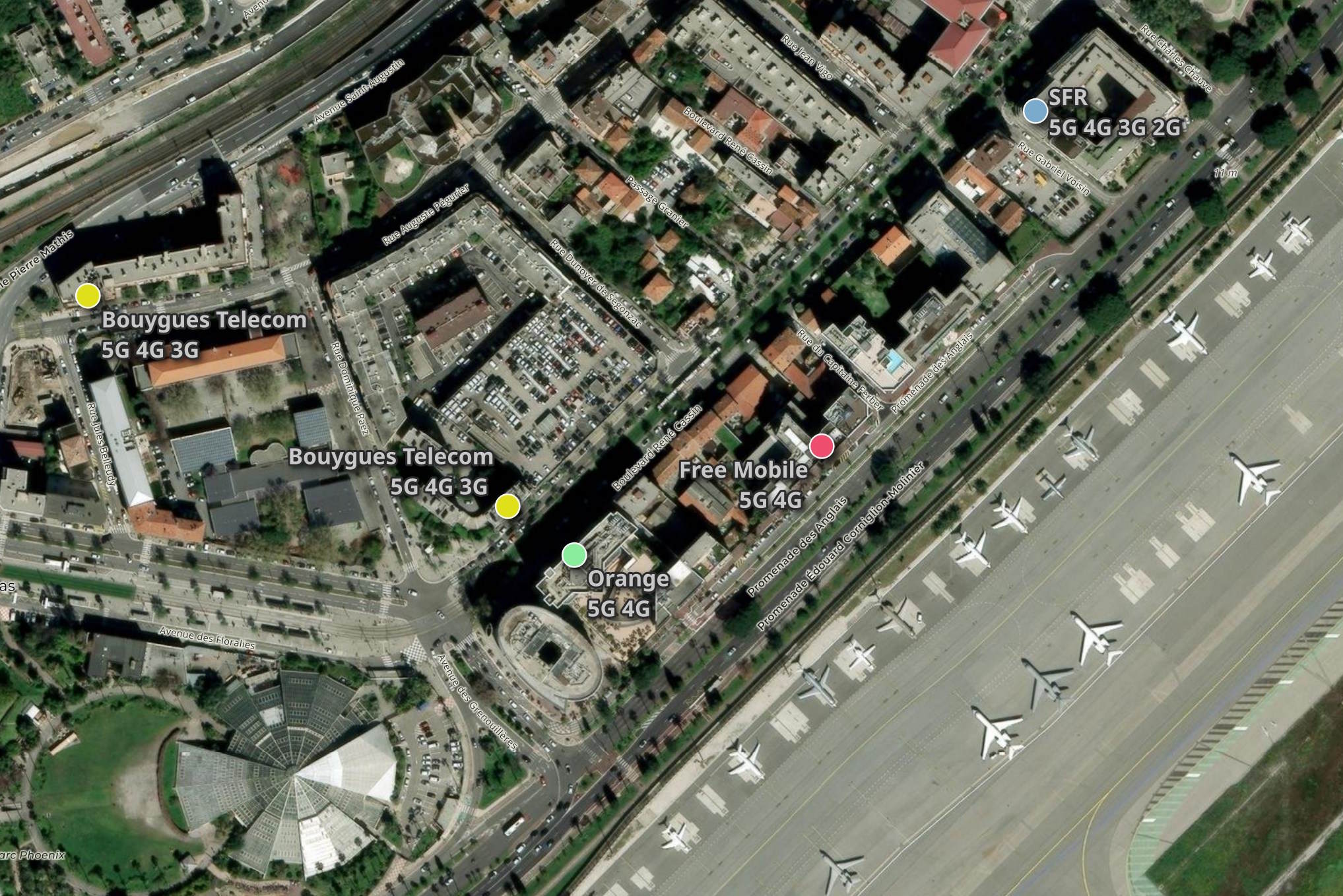
Below are the sites around Nice Airport along with the network generations they support.
Theoretical Coverage Maps
The theoretical coverage dataset has polygons showing each brand's coverage for each quarter going back to 2017. These are broken down by network generation and separated by voice and data.
Below, I'll download this dataset.
$ mkdir -p ~/coverage
$ cd ~/coverage
$ wget -r \
       --no-parent \
       -A 7z \
       https://data.arcep.fr/mobile/couvertures_theoriques/
The resulting set of 7Zip files is 46 GB.
$ du -hs data.arcep.fr/ # 46 GB
These 7Zip files can contain either a GeoDatabase set of files for the older datasets or a GeoPackage (GPKG) file in case of the newer ones. Below, I'll figure out how many contain a GPKG file.
$ python3
from   collections import Counter
import pathlib

import py7zr
from   rich.progress import track


has_gpkg = {}

for x in track(list(pathlib.Path(".").glob("**/*.7z"))):
    try:
        with py7zr.SevenZipFile(x, 'r') as archive:
            has_gpkg[str(x)] = any([True
                                    for y in archive.getnames()
                                    if y.lower().endswith('.gpkg')])
    except Exception as e:
        print(x, e)
Three 7Zip files weren't readable by the above. I'll exclude them from this analysis.
data.arcep.fr/mobile/couvertures_theoriques/2023_T2/Outremer/973_Guyane/2023_T2_couv_973_ORCA_2G_voix.gpkg.7z not a 7z file
data.arcep.fr/mobile/couvertures_theoriques/2023_T2/Outremer/973_Guyane/2023_T2_couv_973_ORCA_3G_data.gpkg.7z not a 7z file
data.arcep.fr/mobile/couvertures_theoriques/2023_T2/Outremer/973_Guyane/2023_T2_couv_973_ORCA_4G_data.gpkg.7z not a 7z file
Of the remaining files, 1,150 contain GPKG files with the remaining containing legacy GeoDatabases.
Counter(has_gpkg.values()).most_common()
[(True, 1150), (False, 1002)]
A variety of projections are used across the GPKG files.
$ gdalsrsinfo \
    -o proj4 \
    2022_T3_couv_971_OMT_4G_data.gpkg
+proj=utm +zone=20 +ellps=GRS80 +towgs84=0,0,0,0,0,0,0 +units=m +no_defs
$ gdalsrsinfo \
    -o proj4 \
    2022_T3_couv_Metropole_BOUY_4G_data.gpkg
+proj=lcc +lat_0=46.5 +lon_0=3 +lat_1=49 +lat_2=44 +x_0=700000 +y_0=6600000 +ellps=GRS80 +towgs84=0,0,0,0,0,0,0 +units=m +no_defs
Neither GeoDatabases nor GPKG files are suitable for distribution and analysis at this scale. Both are row-based formats meant to be easy to edit but at the expense of being very slow to query in comparison to any column-based format.
I'll run the following to convert the GPKG files into Parquet using EPSG:4326 for their projection.
$ python3
import pathlib

import duckdb
import py7zr
from   rich.progress import track
from   shpyx         import run as execute


con = duckdb.connect(database=':memory:')
con.sql('INSTALL spatial; LOAD spatial')
con.sql('INSTALL parquet; LOAD parquet')

sql = """
COPY(SELECT operateur,
            date,
            techno,
            usage,
            niveau,
            dept,
            geometry: ST_FLIPCOORDINATES(ST_TRANSFORM(geom, '%s', 'EPSG:4326'))
     FROM   ST_READ('%s'))
TO '%s' (FORMAT 'PARQUET')
"""

for x in track(list(pathlib.Path(".").glob("**/*.7z"))):
    try:
        with py7zr.SevenZipFile(x, 'r') as archive:
            selective_files = [y
                               for y in archive.getnames()
                               if y.lower().endswith('.gpkg')]

            if selective_files:
                archive.extract(targets=selective_files)

                for y in selective_files:
                    srs = str(execute('gdalsrsinfo -o proj4 %s' % y).stdout).strip()

                    con.sql(sql % (srs, y, str(y) + '.parquet'))
    except Exception as e:
        print(x, e)
The GPKG filenames contain a truncated mobile phone operator brand while their "operateur" column contains their numeric "Public Land Mobile Network" (PLMN) identifier. I'll build a table of these that'll be used in a join later on.
$ ~/duckdb spill.duckdb
CREATE OR REPLACE TABLE brands AS
    SELECT DISTINCT brand: SPLIT_PART(filename, '_', 5),
                    operateur
    FROM   READ_PARQUET('*.gpkg.parquet', filename=true);
Below are the brand and numeric code pairs.
FROM brands;
┌─────────┬───────────┐
│  brand  │ operateur │
│ varchar │   int64   │
├─────────┼───────────┤
│ FREE    │     20815 │
│ ORCA    │     34001 │
│ TELC    │     64703 │
│ SRR     │     64710 │
│ UTS     │     34012 │
│ ZEOP    │     64700 │
│ DIGIC   │     34020 │
│ OF      │     64700 │
│ OMT     │     34002 │
│ FREE    │     20801 │
│ FRCA    │     34020 │
│ ZEOP    │     34001 │
│ ZEOP    │     64704 │
│ DAUPH   │     34008 │
│ OF      │     20801 │
│ TELC    │     64702 │
│ BOUY    │     20820 │
│ FRCA    │     34004 │
│ SFR0    │     20810 │
└─────────┴───────────┘
I'll then merge the 1K+ Parquet files into one for each quarter of each year.
$ for QUARTER in `ls 20*.gpkg.parquet | cut -c1-7 | sort | uniq`; do
      echo $QUARTER
      ~/duckdb \
          -c "SET memory_limit='64GB';" \
          -c "COPY (
                  SELECT   a.*,
                           b.brand,
                           bbox: {'xmin': ST_XMIN(ST_EXTENT(a.geometry)),
                                  'ymin': ST_YMIN(ST_EXTENT(a.geometry)),
                                  'xmax': ST_XMAX(ST_EXTENT(a.geometry)),
                                  'ymax': ST_YMAX(ST_EXTENT(a.geometry))},
                  FROM     '$QUARTER*.gpkg.parquet' a
                  JOIN     brands b ON a.operateur = b.operateur
                  WHERE    ST_X(ST_CENTROID(a.geometry)) IS NOT NULL
                  ORDER BY HILBERT_ENCODE([ST_Y(ST_CENTROID(a.geometry)),
                                           ST_X(ST_CENTROID(a.geometry))]::double[2])
              ) TO 'theoretical_cover.$QUARTER.parquet' (
                      FORMAT 'PARQUET',
                      CODEC  'ZSTD',
                      COMPRESSION_LEVEL 22,
                      ROW_GROUP_SIZE 15000);" \
          spill.duckdb
  done
Below are the resulting Parquet files.
$ du -hcs theoretical_cover.202*.parquet
345M    theoretical_cover.2022_T3.parquet
4.6G    theoretical_cover.2022_T4.parquet
229M    theoretical_cover.2023_T1.parquet
4.0G    theoretical_cover.2023_T2.parquet
238M    theoretical_cover.2023_T3.parquet
3.6G    theoretical_cover.2023_T4.parquet
226M    theoretical_cover.2024_T1.parquet
3.6G    theoretical_cover.2024_T2.parquet
219M    theoretical_cover.2024_T3.parquet
4.8G    theoretical_cover.2024_T4.parquet
1.6G    theoretical_cover.2025_T1.parquet
5.0G    theoretical_cover.2025_T2.parquet
1.6G    theoretical_cover.2025_T3.parquet
5.6G    theoretical_cover.2025_T4.parquet
36G     total
The GPKG format usage only began in the third quarter of 2022 so this Parquet-formatted dataset won't contain data before that.
Below is a breakdown of unique values and NULL coverage across each column for the 2025 data.
$ ~/duckdb
SELECT   column_name,
         column_type[:30],
         null_percentage,
         approx_unique,
         min[:30],
         max[:30]
FROM     (SUMMARIZE
          FROM 'theoretical_cover.2025*.parquet')
ORDER BY LOWER(column_name);
┌─────────────┬────────────────────────────────┬─────────────────┬───────────────┬────────────────────────────────┬────────────────────────────────┐
│ column_name │        column_type[:30]        │ null_percentage │ approx_unique │            min[:30]            │            max[:30]            │
│   varchar   │            varchar             │  decimal(9,2)   │     int64     │            varchar             │            varchar             │
├─────────────┼────────────────────────────────┼─────────────────┼───────────────┼────────────────────────────────┼────────────────────────────────┤
│ bbox        │ STRUCT(xmin DOUBLE, ymin DOUBL │            0.00 │          9828 │ {'xmin': -63.1531358, 'ymin':  │ {'xmin': 55.276453316344025, ' │
│ brand       │ VARCHAR                        │            0.00 │            15 │ BOUY                           │ ZEOP                           │
│ date        │ VARCHAR                        │            0.00 │             4 │ 2025-03-31                     │ 2025-12-31                     │
│ dept        │ VARCHAR                        │            0.00 │           105 │ 01                             │ 978                            │
│ geometry    │ GEOMETRY('OGC:CRS84')          │            0.00 │         10597 │ POLYGON ((2.333099900266716 48 │ MULTIPOLYGON (((3.389827530127 │
│ niveau      │ VARCHAR                        │            0.00 │             4 │                                │ TBC                            │
│ operateur   │ BIGINT                         │            0.00 │            13 │ 20801                          │ 64710                          │
│ techno      │ VARCHAR                        │            0.00 │             5 │ 2G                             │ 5G                             │
│ usage       │ VARCHAR                        │            0.00 │             1 │ data                           │ voix                           │
└─────────────┴────────────────────────────────┴─────────────────┴───────────────┴────────────────────────────────┴────────────────────────────────┘
Coverage is broken down by mobile network generation as well as data and voice (French: voix) support. These are the row counts for each.
Note: data coverage isn't collected for older generations and voice coverage isn't collected for newer generations.
WITH a AS (
    SELECT   techno,
             usage,
             cnt: COUNT(*)
    FROM     'theoretical_cover.*.parquet'
    GROUP BY 1, 2
)
PIVOT a
ON       usage
USING    SUM(cnt)
GROUP BY techno
ORDER BY techno;
┌─────────┬────────┬────────┐
│ techno  │  data  │  voix  │
│ varchar │ int128 │ int128 │
├─────────┼────────┼────────┤
│ 2G      │   NULL │ 861398 │
│ 2G3G    │   NULL │ 924737 │
│ 3G      │  51345 │   NULL │
│ 4G      │ 154727 │   NULL │
│ 5G      │    480 │   NULL │
└─────────┴────────┴────────┘
Below are the changes in 4G data coverage area broken down by brand and quarter of reporting.
.maxrows 100

SELECT   brand,
         date,
         area: ROUND(SUM(ST_AREA(geometry)), 4)
FROM     'theoretical_cover.2025*.parquet'
WHERE    techno = '4G'
AND      usage  = 'data'
GROUP BY 1, 2
ORDER BY 1, 2;
┌─────────┬────────────┬──────────┐
│  brand  │    date    │   area   │
│ varchar │  varchar   │  double  │
├─────────┼────────────┼──────────┤
│ BOUY    │ 2025-03-31 │  61.8234 │
│ BOUY    │ 2025-06-30 │   61.868 │
│ BOUY    │ 2025-09-30 │  61.9096 │
│ BOUY    │ 2025-12-31 │  61.8935 │
│ DAUPH   │ 2025-03-31 │   0.0051 │
│ DAUPH   │ 2025-06-30 │   0.0052 │
│ DAUPH   │ 2025-09-30 │   0.0052 │
│ DAUPH   │ 2025-12-31 │   0.0052 │
│ DIGIC   │ 2025-03-31 │   0.4977 │
│ DIGIC   │ 2025-06-30 │   0.4079 │
│ DIGIC   │ 2025-09-30 │    0.407 │
│ DIGIC   │ 2025-12-31 │    0.411 │
│ FRCA    │ 2025-03-31 │    0.796 │
│ FRCA    │ 2025-06-30 │   0.7558 │
│ FRCA    │ 2025-09-30 │   0.7559 │
│ FRCA    │ 2025-12-31 │   0.7599 │
│ FREE    │ 2025-03-31 │ 121.0205 │
│ FREE    │ 2025-06-30 │ 121.1464 │
│ FREE    │ 2025-09-30 │ 121.5269 │
│ FREE    │ 2025-12-31 │ 124.2319 │
│ OF      │ 2025-03-31 │  62.0904 │
│ OF      │ 2025-06-30 │  62.1185 │
│ OF      │ 2025-09-30 │  62.4091 │
│ OF      │ 2025-12-31 │   62.372 │
│ OMT     │ 2025-03-31 │   0.5476 │
│ OMT     │ 2025-06-30 │   0.5496 │
│ OMT     │ 2025-09-30 │   0.5528 │
│ OMT     │ 2025-12-31 │   0.5584 │
│ ORCA    │ 2025-03-31 │   0.5986 │
│ ORCA    │ 2025-06-30 │   0.5867 │
│ ORCA    │ 2025-09-30 │   0.5867 │
│ ORCA    │ 2025-12-31 │   0.5861 │
│ SFR0    │ 2025-03-31 │  62.3481 │
│ SFR0    │ 2025-06-30 │  62.4215 │
│ SFR0    │ 2025-09-30 │  62.4297 │
│ SFR0    │ 2025-12-31 │  62.4926 │
│ SRR     │ 2025-03-31 │   0.2295 │
│ SRR     │ 2025-06-30 │   0.2287 │
│ SRR     │ 2025-09-30 │   0.2287 │
│ SRR     │ 2025-12-31 │   0.2285 │
│ TELC    │ 2025-03-31 │   0.1628 │
│ TELC    │ 2025-06-30 │   0.1704 │
│ TELC    │ 2025-09-30 │   0.1731 │
│ TELC    │ 2025-12-31 │   0.1731 │
│ UTS     │ 2025-03-31 │   0.0026 │
│ UTS     │ 2025-09-30 │   0.0052 │
│ ZEOP    │ 2025-03-31 │   1.0214 │
│ ZEOP    │ 2025-06-30 │    1.307 │
│ ZEOP    │ 2025-09-30 │   1.0065 │
│ ZEOP    │ 2025-12-31 │   1.0079 │
└─────────┴────────────┴──────────┘
I'll extract Free's 4G data coverage for the end of 2025.
COPY (
    FROM  'theoretical_cover.2025*.parquet'
    WHERE techno = '4G'
    AND   usage  = 'data'
    AND   date   = '2025-12-31'
    AND   brand  = 'FREE'
) TO 'tc.free.parquet' (
      FORMAT 'PARQUET',
      CODEC  'ZSTD',
      COMPRESSION_LEVEL 22,
      ROW_GROUP_SIZE 15000);
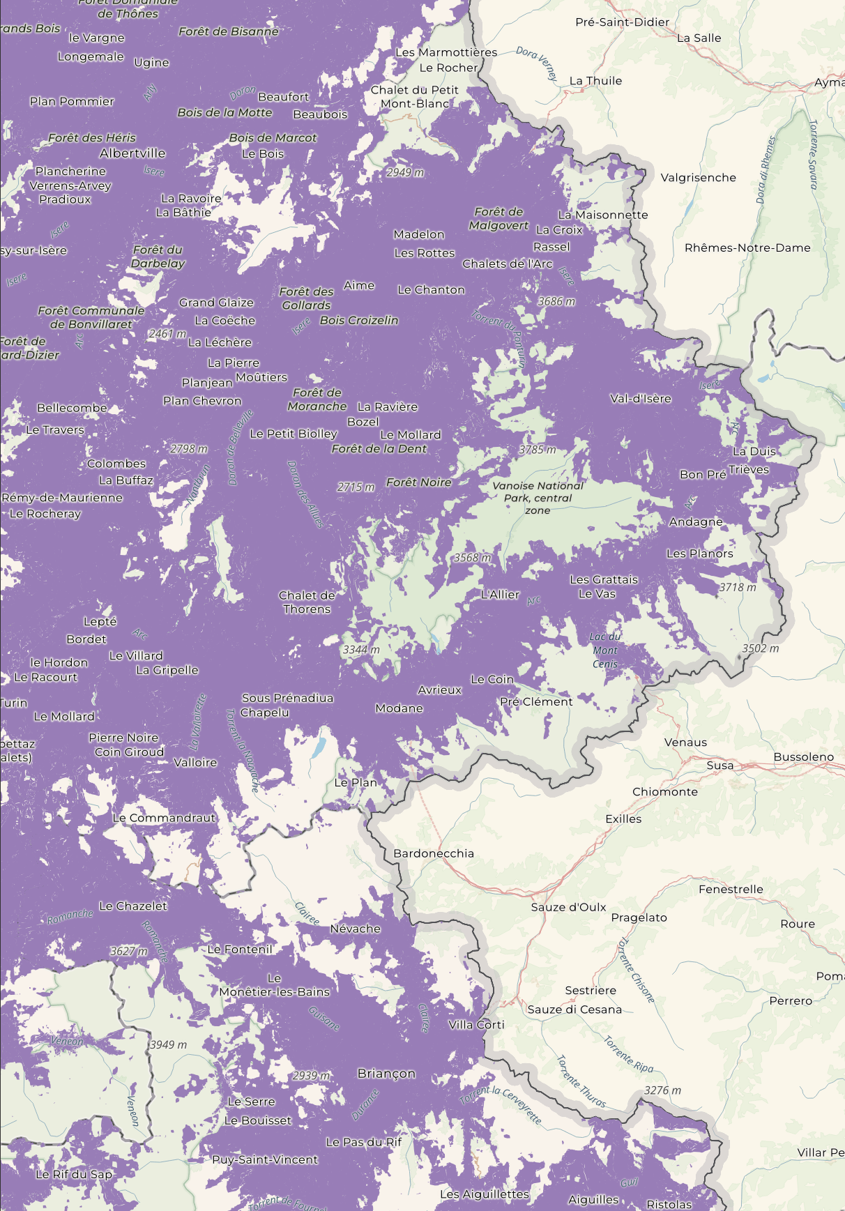
Most of France is well-covered.
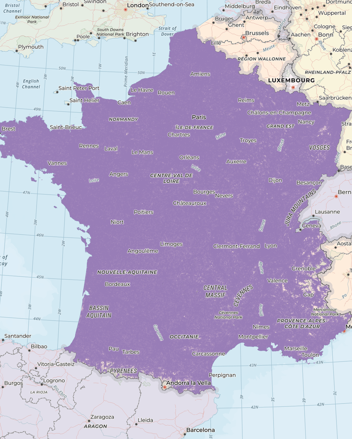
When zooming in on the Alps, you can see gaps where there isn't any coverage.
Ookla & Speedchecker
Since 2022, crowd-sourced speed measurements have been included in these datasets. The last quarter of 2025 has measurements from both Ookla and Speedchecker.
I'll first import Ookla's data into a DuckDB table.
$ ~/duckdb
CREATE OR REPLACE TABLE a AS
    SELECT * EXCLUDE(date_time_start,
                     latitude_start,
                     longitude_start,
                     protocole),
            started_at: STRPTIME(date_time_start, '%d/%m/%Y %H:%M:%S.%g'),
            geom:       ST_POINT(longitude_start, latitude_start)
    FROM '2025_T4_crowd_Ookla.csv';
There are almost ~430K rows in this table.
SELECT COUNT(*) FROM a; -- 428851
Below are the field names, data types, percentages of NULLs per column, number of unique values and minimum and maximum values for each column.
Several columns only contain NULLs so I've excluded them from this query.
SELECT   column_name,
         column_type[:30],
         null_percentage,
         approx_unique,
         min[:30],
         max[:30]
FROM     (SUMMARIZE
          FROM a)
WHERE    null_percentage < 100
ORDER BY LOWER(column_name);
┌─────────────┬──────────────────┬─────────────────┬───────────────┬─────────────────────┬─────────────────────┐
│ column_name │ column_type[:30] │ null_percentage │ approx_unique │      min[:30]       │      max[:30]       │
│   varchar   │     varchar      │  decimal(9,2)   │     int64     │       varchar       │       varchar       │
├─────────────┼──────────────────┼─────────────────┼───────────────┼─────────────────────┼─────────────────────┤
│ bitrate_dl  │ DOUBLE           │            0.00 │        265709 │ 0.001               │ 1810.234            │
│ geom        │ GEOMETRY         │            0.00 │         50624 │ POINT (0 44.58)     │ POINT (-1.81 48.34) │
│ mcc_start   │ BIGINT           │            0.00 │             3 │ 208                 │ 647                 │
│ mnc_start   │ VARCHAR          │            0.00 │             6 │ 01                  │ 20                  │
│ operator    │ VARCHAR          │            0.00 │             5 │ Bouygues            │ SRR                 │
│ started_at  │ TIMESTAMP        │            0.00 │        425630 │ 2025-10-01 02:00:22 │ 2026-01-01 00:59:34 │
└─────────────┴──────────────────┴─────────────────┴───────────────┴─────────────────────┴─────────────────────┘
Below are the number of measurements for each month broken down by operator.
WITH a AS (
    SELECT   operator,
             yyyy_mm: STRFTIME(started_at, '%Y-%m'),
             cnt:     COUNT(*)
    FROM     a
    GROUP BY 1, 2
)
PIVOT    a
ON       operator
USING    SUM(cnt)
GROUP BY yyyy_mm
ORDER BY yyyy_mm;
┌─────────┬──────────┬────────┬────────┬────────┬────────┐
│ yyyy_mm │ Bouygues │  Free  │ Orange │  SFR   │  SRR   │
│ varchar │  int128  │ int128 │ int128 │ int128 │ int128 │
├─────────┼──────────┼────────┼────────┼────────┼────────┤
│ 2025-10 │    32928 │  42820 │  51075 │  13862 │      3 │
│ 2025-11 │    32571 │  40649 │  49487 │  15334 │      6 │
│ 2025-12 │    37163 │  44794 │  52850 │  15148 │     11 │
│ 2026-01 │       31 │     47 │     50 │     22 │   NULL │
└─────────┴──────────┴────────┴────────┴────────┴────────┘
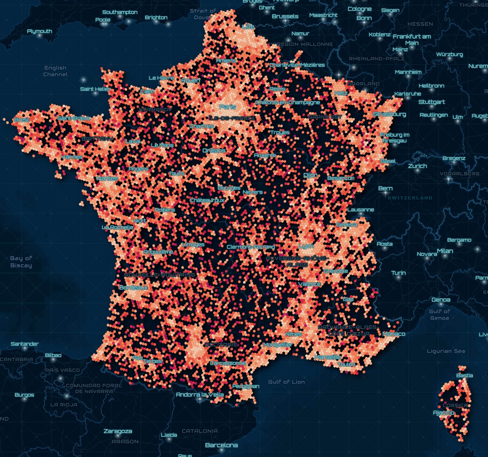
I'll create a heatmap of the highest measurements seen for each operator.
CREATE OR REPLACE TABLE h3_stats AS
    SELECT   h3_3: H3_LATLNG_TO_CELL(
                       ST_Y(geom),
                       ST_X(geom),
                       6),
             operator,
             bitrate_dl: MAX(bitrate_dl)
    FROM     a
    GROUP BY 1, 2;

COPY (
    SELECT geometry: ST_ASWKB(H3_CELL_TO_BOUNDARY_WKT(h3_3)::geometry),
           operator,
           bitrate_dl
    FROM   h3_stats
    WHERE  ST_XMIN(H3_CELL_TO_BOUNDARY_WKT(h3_3)::geometry) BETWEEN -179 AND 179
    AND    ST_XMAX(H3_CELL_TO_BOUNDARY_WKT(h3_3)::geometry) BETWEEN -179 AND 179
) TO 'ookla.h3_3_stats.parquet' (
        FORMAT 'PARQUET',
        CODEC  'ZSTD',
        COMPRESSION_LEVEL 22,
        ROW_GROUP_SIZE 15000);
The brightest hexagons below show where Orange's highest speeds were seen in this dataset.
Speedchecker's measurements are further broken down by device and also include an upload speed measurement. Below, I'll import their results from the end of last year into a DuckDB table.
$ ~/duckdb
CREATE OR REPLACE TABLE a AS
    SELECT * EXCLUDE(latitude_start,
                     longitude_start),
           geom: ST_POINT(longitude_start, latitude_start)
    FROM   '2025_T4_crowd_Speedchecker.csv';
This dataset has over 51K records.
SELECT COUNT(*) FROM a; -- 51594
Below are the field names, data types, percentages of NULLs per column, number of unique values and minimum and maximum values for each column.
Several columns only contain NULLs so I've excluded them from this query.
SELECT   column_name,
         column_type[:30],
         null_percentage,
         approx_unique,
         min[:30],
         max[:30]
FROM     (SUMMARIZE
          FROM a)
WHERE    null_percentage < 100
ORDER BY LOWER(column_name);
┌─────────────┬──────────────────┬─────────────────┬───────────────┬─────────────────┬────────────────────────────┐
│ column_name │ column_type[:30] │ null_percentage │ approx_unique │    min[:30]     │          max[:30]          │
│   varchar   │     varchar      │  decimal(9,2)   │     int64     │     varchar     │          varchar           │
├─────────────┼──────────────────┼─────────────────┼───────────────┼─────────────────┼────────────────────────────┤
│ bitrate_dl  │ DOUBLE           │            0.02 │         48321 │ 0.01            │ 1491.45                    │
│ bitrate_ul  │ DOUBLE           │           31.64 │         18354 │ 0.008           │ 249.076                    │
│ geom        │ GEOMETRY         │            0.00 │         45497 │ POINT (2 48.31) │ POINT (1.5921199 49.04092) │
│ mcc_start   │ BIGINT           │            0.00 │             1 │ 208             │ 208                        │
│ mnc_start   │ BIGINT           │            0.00 │             4 │ 1               │ 20                         │
│ operator    │ VARCHAR          │            0.00 │             4 │ Bouygues        │ SFR                        │
│ protocole   │ VARCHAR          │            0.00 │             1 │ DOWNLOAD        │ DOWNLOAD                   │
│ terminal    │ VARCHAR          │            5.19 │          1346 │ 2112123AG       │ vivo Y76 5G                │
└─────────────┴──────────────────┴─────────────────┴───────────────┴─────────────────┴────────────────────────────┘
Below are the fastest download speeds seen on each network along with the device the speed was seen with.
WITH b AS (
    WITH a AS (
        SELECT   operator,
                 terminal,
                 bitrate_dl
        FROM     a
        GROUP BY 1, 2, 3
        ORDER BY 3 DESC
    )
    SELECT *,
           ROW_NUMBER() OVER (PARTITION BY operator
                              ORDER BY     bitrate_dl DESC) AS rn
    FROM   a
)
SELECT   operator,
         terminal,
         bitrate_dl
FROM     b
WHERE    rn = 1
ORDER BY bitrate_dl DESC;
┌──────────┬────────────────────┬────────────┐
│ operator │      terminal      │ bitrate_dl │
│ varchar  │      varchar       │   double   │
├──────────┼────────────────────┼────────────┤
│ Orange   │ Galaxy S23         │    1491.45 │
│ SFR      │ Galaxy Z Flip5     │   1457.584 │
│ Bouygues │ Samsung Galaxy A54 │     1002.3 │
│ Free     │ Samsung Galaxy A54 │     895.83 │
└──────────┴────────────────────┴────────────┘
Quality of Service
The Quality of Service files are broken down by year, separated by voice and data and also separated by measurements taken while stationary or while moving. I'll load the stationary data measurements for Metropolitan France into DuckDB.
$ ~/duckdb
CREATE OR REPLACE TABLE a AS
    SELECT * EXCLUDE(bitrate_dl,
                     bitrate_ul,
                     acess_duration,
                     date_start,
                     hour_start,
                     latitude_start,
                     longitude_start,
                     loaded_in_less_10_secondes,
                     loaded_in_less_5_secondes,
                     quality_correct,
                     quality_perfect,
                     upload_ok,
                     situation),
           bitrate_dl: REPLACE(bitrate_dl, ',', '.')::DOUBLE,
           bitrate_ul: REPLACE(bitrate_ul, ',', '.')::DOUBLE,
           acess_duration: REPLACE(acess_duration, ',', '.')::DOUBLE,
           started_at: CONCAT(date_start, ' ', hour_start)::TIMESTAMP,
           geom: ST_POINT(longitude_start, latitude_start),
           loaded_in_less_10_secondes: loaded_in_less_10_secondes::BOOLEAN,
           loaded_in_less_5_secondes: loaded_in_less_5_secondes::BOOLEAN,
           quality_correct: quality_correct::BOOLEAN,
           quality_perfect: quality_perfect::BOOLEAN,
           upload_ok: upload_ok::BOOLEAN,
           situation: LOWER(situation)
    FROM READ_CSV('2025_QoS_Metropole_data_habitations.csv',
                  delim=';',
                  ignore_errors=true);
This table has over 273K rows.
SELECT COUNT(*) FROM a; -- 273710
Below are the field names, data types, percentages of NULLs per column, number of unique values and minimum and maximum values for each column.
Several columns only contain NULLs so I've excluded them from this query.
SELECT   column_name,
         column_type[:30],
         null_percentage,
         approx_unique,
         min[:30],
         max[:30]
FROM     (SUMMARIZE
          FROM a)
WHERE    null_percentage < 100
ORDER BY LOWER(column_name);
┌────────────────────────────┬──────────────────┬─────────────────┬───────────────┬────────────────────────────────┬────────────────────────────────┐
│        column_name         │ column_type[:30] │ null_percentage │ approx_unique │            min[:30]            │            max[:30]            │
│          varchar           │     varchar      │  decimal(9,2)   │     int64     │            varchar             │            varchar             │
├────────────────────────────┼──────────────────┼─────────────────┼───────────────┼────────────────────────────────┼────────────────────────────────┤
│ acess_duration             │ DOUBLE           │            5.17 │          2252 │ 0.0                            │ 66.02                          │
│ bitrate_dl                 │ DOUBLE           │           90.57 │         14847 │ 0.0                            │ 993.9109005                    │
│ bitrate_ul                 │ DOUBLE           │           95.29 │         10844 │ 0.0                            │ 155.9220818                    │
│ geom                       │ GEOMETRY         │            0.00 │         73125 │ POINT (2.125 48.6238)          │ POINT (5.73514 45.08009)       │
│ insee_com                  │ BIGINT           │            0.00 │          1245 │ 1043                           │ 95678                          │
│ loaded_in_less_10_secondes │ BOOLEAN          │           28.53 │             2 │ false                          │ true                           │
│ loaded_in_less_5_secondes  │ BOOLEAN          │           28.53 │             2 │ false                          │ true                           │
│ mcc_start                  │ BIGINT           │           11.49 │             3 │ 0                              │ 214                            │
│ mnc_start                  │ BIGINT           │           11.49 │            11 │ 0                              │ 88                             │
│ operator                   │ VARCHAR          │            0.00 │             4 │ Bouygues                       │ SFR                            │
│ protocole                  │ VARCHAR          │            0.00 │             6 │ DOWNLOAD                       │ WEB                            │
│ quality_correct            │ BOOLEAN          │           95.22 │             2 │ false                          │ true                           │
│ quality_perfect            │ BOOLEAN          │           95.22 │             2 │ false                          │ true                           │
│ Result_1                   │ VARCHAR          │            0.00 │             5 │ Drop                           │ Traffic Fail                   │
│ rscp                       │ DOUBLE           │           98.03 │          2485 │ -121.0                         │ -38.89                         │
│ rsrp                       │ DOUBLE           │            4.38 │          6304 │ -154.33                        │ -53.67                         │
│ rsrq                       │ DOUBLE           │            4.23 │          2044 │ -30.0                          │ -1.16                          │
│ situation                  │ VARCHAR          │            0.00 │             3 │ incar                          │ outdoor                        │
│ started_at                 │ TIMESTAMP        │            0.00 │        161212 │ 2025-05-26 08:20:12            │ 2025-08-29 18:09:16            │
│ techno_start               │ VARCHAR          │            0.00 │             1 │ 5G                             │ 5G                             │
│ terminal                   │ VARCHAR          │            0.00 │             3 │ SM-F731B                       │ SM-S921B                       │
│ territory                  │ VARCHAR          │            0.00 │             1 │ METROPOLE                      │ METROPOLE                      │
│ transfert_file_size        │ BIGINT           │           81.14 │             3 │ 1                              │ 250                            │
│ upload_ok                  │ BOOLEAN          │           95.28 │             2 │ false                          │ true                           │
│ url                        │ VARCHAR          │            9.67 │            32 │ https://fr.linkedin.com        │ https://x.com/?locale=fr       │
│ zone                       │ VARCHAR          │            0.00 │             4 │ Zones denses                   │ Zones touristiques             │
│ zone_name                  │ VARCHAR          │            0.00 │          1175 │ Abbaye du Mont-Saint-Michel Mo │ Zoo parc de Beauval Saint-Aign │
└────────────────────────────┴──────────────────┴─────────────────┴───────────────┴────────────────────────────────┴────────────────────────────────┘
These are the measurement counts for each operator for each month.
WITH a AS (
    SELECT   operator,
             yyyy_mm: STRFTIME(started_at, '%Y-%m'),
             cnt:     COUNT(*)
    FROM     a
    GROUP BY 1, 2
)
PIVOT    a
ON       operator
USING    SUM(cnt)
GROUP BY yyyy_mm
ORDER BY yyyy_mm;
┌─────────┬──────────┬────────┬────────┬────────┐
│ yyyy_mm │ Bouygues │  Free  │ Orange │  SFR   │
│ varchar │  int128  │ int128 │ int128 │ int128 │
├─────────┼──────────┼────────┼────────┼────────┤
│ 2025-05 │      949 │    939 │    950 │    948 │
│ 2025-06 │    19349 │  19182 │  19346 │  19226 │
│ 2025-07 │    29692 │  29898 │  30012 │  29998 │
│ 2025-08 │    18259 │  18245 │  18374 │  18343 │
└─────────┴──────────┴────────┴────────┴────────┘
There are three different types of situations that tests can fall under.
SELECT   situation,
         count(*)
FROM     a
GROUP BY 1;
┌───────────┬──────────────┐
│ situation │ count_star() │
│  varchar  │    int64     │
├───────────┼──────────────┤
│ indoor    │       104322 │
│ outdoor   │       104231 │
│ incar     │        65157 │
└───────────┴──────────────┘
These are the test result counts for each operator.
WITH a AS (
    SELECT   operator,
             Result_1,
             cnt:     COUNT(*)
    FROM     a
    GROUP BY 1, 2
)
PIVOT    a
ON       operator
USING    SUM(cnt)
GROUP BY Result_1
ORDER BY Result_1;
┌──────────────┬──────────┬────────┬────────┬────────┐
│   Result_1   │ Bouygues │  Free  │ Orange │  SFR   │
│   varchar    │  int128  │ int128 │ int128 │ int128 │
├──────────────┼──────────┼────────┼────────┼────────┤
│ Drop         │      445 │    802 │    479 │    399 │
│ Setup Fail   │       12 │      9 │      8 │      9 │
│ Success      │    56651 │  54544 │  59420 │  56466 │
│ TimeOut      │     3988 │   4868 │   2841 │   4270 │
│ Traffic Fail │     7153 │   8041 │   5934 │   7371 │
└──────────────┴──────────┴────────┴────────┴────────┘
Below are the top 30 operator-url pair counts where there was anything other than a successful test.
SELECT   operator,
         url,
         COUNT(*)
FROM     a
WHERE    Result_1 != 'Success'
AND      url IS NOT NULL
GROUP BY 1, 2
ORDER BY 3 DESC
LIMIT    30;
┌──────────┬──────────────────────────────────────────────────┬──────────────┐
│ operator │                       url                        │ count_star() │
│ varchar  │                     varchar                      │    int64     │
├──────────┼──────────────────────────────────────────────────┼──────────────┤
│ Free     │ https://test-debit7-v6.afdtech.com               │         3146 │
│ SFR      │ https://test-debit7-v6.afdtech.com               │         2977 │
│ Bouygues │ https://test-debit7-v6.afdtech.com               │         2952 │
│ Orange   │ https://test-debit7-v6.afdtech.com               │         2643 │
│ Free     │ https://test-debit7-v6.afdtech.com/250Mo.bin     │         2364 │
│ Free     │ https://test-debit8-v6.afdtech.com/250Mo.bin     │         2168 │
│ SFR      │ https://test-debit7-v6.afdtech.com/250Mo.bin     │         2031 │
│ SFR      │ https://test-debit8-v6.afdtech.com/250Mo.bin     │         1980 │
│ Bouygues │ https://test-debit7-v6.afdtech.com/250Mo.bin     │         1933 │
│ Bouygues │ https://test-debit8-v6.afdtech.com/250Mo.bin     │         1877 │
│ Orange   │ https://test-debit7-v6.afdtech.com/250Mo.bin     │         1492 │
│ Orange   │ https://test-debit8-v6.afdtech.com/250Mo.bin     │         1492 │
│ Free     │ https://www.messervices.etudiant.gouv.fr/envole/ │          298 │
│ Bouygues │ https://www.messervices.etudiant.gouv.fr/envole/ │          289 │
│ Free     │ https://www.marmiton.org/recettes                │          273 │
│ Free     │ https://www.francetravail.fr/accueil/            │          249 │
│ Free     │ https://recherche.lefigaro.fr/recherche/         │          247 │
│ Free     │ https://www.index-education.com/fr/              │          243 │
│ Free     │ https://www.doctolib.fr/                         │          243 │
│ Free     │ https://www.tiktok.com/                          │          241 │
│ SFR      │ https://www.messervices.etudiant.gouv.fr/envole/ │          233 │
│ Orange   │ https://www.messervices.etudiant.gouv.fr/envole/ │          231 │
│ Free     │ https://redditinc.com/                           │          231 │
│ Bouygues │ https://redditinc.com/                           │          226 │
│ SFR      │ https://www.marmiton.org/recettes                │          222 │
│ Free     │ https://www.ubereats.com/fr                      │          217 │
│ Bouygues │ https://www.doctolib.fr/                         │          216 │
│ Bouygues │ https://www.francetravail.fr/accueil/            │          205 │
│ SFR      │ https://www.index-education.com/fr/              │          203 │
│ SFR      │ https://www.tiktok.com/                          │          200 │
└──────────┴──────────────────────────────────────────────────┴──────────────┘