Digital Earth Australia's Tidal Composites dataset is a cloud-free mosaic of Australia’s coasts, estuaries and reefs at low and high tide. These were built off of Sentinel-2 satellite imagery, covering 2016 till 2023 and total ~2.6 TB in GeoTIFF format. These are being hosted on AWS S3.
The Sentinel-2 constellation is made up of three satellites that capture 10-meter imagery across 13-spectral bands. The European Space Agency launched in the first satellite in 2015, the second in 2017 and the third in September of last year.
Below is a high-tide, blue-band image taken of Hervey Bay, Queensland in 2023. It's coloured with a rainbow colour ramp.
In this post, I'll explore the Tidal Composites dataset.
My Workstation
I'm using a 5.7 GHz AMD Ryzen 9 9950X CPU. It has 16 cores and 32 threads and 1.2 MB of L1, 16 MB of L2 and 64 MB of L3 cache. It has a liquid cooler attached and is housed in a spacious, full-sized Cooler Master HAF 700 computer case.
The system has 96 GB of DDR5 RAM clocked at 4,800 MT/s and a 5th-generation, Crucial T700 4 TB NVMe M.2 SSD which can read at speeds up to 12,400 MB/s. There is a heatsink on the SSD to help keep its temperature down. This is my system's C drive.
The system is powered by a 1,200-watt, fully modular Corsair Power Supply and is sat on an ASRock X870E Nova 90 Motherboard.
I'm running Ubuntu 24 LTS via Microsoft's Ubuntu for Windows on Windows 11 Pro. In case you're wondering why I don't run a Linux-based desktop as my primary work environment, I'm still using an Nvidia GTX 1080 GPU which has better driver support on Windows and ArcGIS Pro only supports Windows natively.
Installing Prerequisites
I'll use Python 3.12.3, GDAL 3.9.3 and a few other tools to help analyse the data in this post.
$ sudo add-apt-repository ppa:deadsnakes/ppa
$ sudo add-apt-repository ppa:ubuntugis/ubuntugis-unstable
$ sudo apt update
$ sudo apt install \
    gdal-bin \
    jq \
    python3-pip \
    python3.12-venv
I'll set up a Python Virtual Environment and install the latest version of the AWS CLI toolkit.
$ python3 -m venv ~/.aus
$ source ~/.aus/bin/activate
$ python -m pip install awscli
I'll use DuckDB v1.4.1, along with its H3, JSON, Lindel, Parquet and Spatial extensions, in this post.
$ cd ~
$ wget -c https://github.com/duckdb/duckdb/releases/download/v1.4.1/duckdb_cli-linux-amd64.zip
$ unzip -j duckdb_cli-linux-amd64.zip
$ chmod +x duckdb
$ ~/duckdb
INSTALL h3 FROM community;
INSTALL lindel FROM community;
INSTALL json;
INSTALL parquet;
INSTALL spatial;
I'll set up DuckDB to load every installed extension each time it launches.
$ vi ~/.duckdbrc
.timer on
.width 180
LOAD h3;
LOAD lindel;
LOAD json;
LOAD parquet;
LOAD spatial;
The maps in this post were rendered using QGIS version 3.44. QGIS is a desktop application that runs on Windows, macOS and Linux. The application has grown in popularity in recent years and has ~15M application launches from users all around the world each month.
I used QGIS' Tile+ plugin to add basemaps from Bing to the maps in this post.
Analysis-Ready Metadata
I'll download the list of files and their respective metadata from S3. The following produced a 325,557-line, 140 MB JSONL file.
$ mkdir -p ~/dea
$ cd ~/dea

$ aws --no-sign-request \
      --output json \
      s3api \
      list-objects \
      --bucket dea-public-data \
      --max-items=1000000000 \
      --prefix=derivative/ga_s2_tidal_composites_cyear_3 \
    | jq -c '.Contents[]' \
    > dea.s3.json
I'll build a DuckDB table from the JSONL file to help analyse the file listing.
$ ~/duckdb dea.duckdb
CREATE OR REPLACE TABLE s3 AS
    SELECT *,
           LOWER(SPLIT(SPLIT(SPLIT(Key, '/')[7], '_')[-1], '.')[-1]) AS format,
           REPLACE(SPLIT(Key, '/')[4], 'x', '')::INT AS x,
           REPLACE(SPLIT(Key, '/')[5], 'y', '')::INT AS y,
           SPLIT(SPLIT(SPLIT(SPLIT(Key, '/')[7], '_')[-1], '.')[1], '-')[1] AS tide,
           REPLACE(REPLACE(SPLIT(SPLIT(SPLIT(Key, '/')[7], '_')[-1], '.')[1], 'high-', ''), 'low-', '') AS band,
           SPLIT(SPLIT(Key, '/')[6], '-')[1]::INT AS year
    FROM   READ_JSON('dea.s3.json')
    WHERE  SPLIT(Key, '/')[6] LIKE '20%--P1Y'
    AND    SPLIT(SPLIT(SPLIT(SPLIT(Key, '/')[7], '_')[-1], '.')[1], '-')[1] != 'qa';
Below is an example record from the table created above.
$ echo "SELECT * EXCLUDE(Owner),
               Owner::JSON AS Owner
        FROM   s3
        WHERE  format = 'tif'
        LIMIT  1" \
    | ~/duckdb -json dea.duckdb \
    | jq -S .
[
  {
    "ChecksumAlgorithm": "[CRC32]",
    "ChecksumType": "COMPOSITE",
    "ETag": "\"4953d4e03bd4795567419b9a02b3fc53-2\"",
    "Key": "derivative/ga_s2_tidal_composites_cyear_3/1-0-0/x078/y124/2016--P1Y/ga_s2_tidal_composites_cyear_3_x078y124_2016--P1Y_final_high-blue.tif",
    "LastModified": "2025-05-06T08:42:43.000Z",
    "Owner": {
      "DisplayName": null,
      "ID": "aa1c69e19883ec24c399e75c3b2ee0812828dccf66574abf4ad7a91767cdb3fa"
    },
    "Size": 11535601,
    "StorageClass": "INTELLIGENT_TIERING",
    "band": "blue",
    "format": "tif",
    "tide": "high",
    "x": 78,
    "y": 124,
    "year": 2016
  }
]
Cloud-Optimised GeoTIFFs
There's ~2.6 TB of content in this dataset with the vast majority being made up of GeoTIFF images. Below are the number of MBs for each file format broken down by year.
$ ~/duckdb dea.duckdb
PIVOT    s3
ON       format
USING    ROUND(SUM(Size) / 1024 ** 2)::INT
GROUP BY year
ORDER BY year;
┌───────┬───────┬───────┬───────┬───────┬────────┬───────┐
│ year  │  jpg  │ json  │  png  │ sha1  │  tif   │ yaml  │
│ int32 │ int32 │ int32 │ int32 │ int32 │ int32  │ int32 │
├───────┼───────┼───────┼───────┼───────┼────────┼───────┤
│  2016 │    12 │    21 │    29 │     3 │ 254858 │    11 │
│  2017 │    17 │    36 │    45 │     4 │ 358245 │    23 │
│  2018 │    17 │    42 │    48 │     4 │ 354476 │    29 │
│  2019 │    17 │    46 │    50 │     4 │ 353264 │    33 │
│  2020 │    16 │    46 │    50 │     4 │ 354057 │    33 │
│  2021 │    16 │    44 │    49 │     4 │ 354838 │    31 │
│  2022 │    16 │    43 │    49 │     4 │ 353765 │    30 │
│  2023 │    16 │    43 │    49 │     4 │ 351874 │    30 │
└───────┴───────┴───────┴───────┴───────┴────────┴───────┘
I'll download a tile's worth of GeoTIFFs and other metadata.
$ aws s3 sync \
    s3://dea-public-data/derivative/ga_s2_tidal_composites_cyear_3/1-0-0/x202/y125/2023--P1Y/ \
    ./ \
    --no-sign-request
The GeoTIFFs are Cloud-Optimised GeoTIFF containers. They contain Tiled Multi-Resolution TIFFs / Tiled Pyramid TIFFs. This means there are several versions of the same image at different resolutions within the TIFF file. The largest image within any one GeoTIFF is 3200 x 3200-pixels.
$ gdalinfo -json \
    ga_s2_tidal_composites_cyear_3_x202y125_2023--P1Y_final_high-blue.tif \
    | jq -S '.size'
[
  3200,
  3200
]
These files are structured so it's easy to only read a portion of a file for any one resolution you're interested in. A file might be 10s or 100s of MB but a JavaScript-based Web Application might only need to download ~2 MB of data from that file in order to render its lowest resolution.
Below you can see there are 1600x1600, 800x800, etc.. versions of the image within a single GeoTIFF file.
$ gdalinfo -json \
    ga_s2_tidal_composites_cyear_3_x202y125_2023--P1Y_final_high-blue.tif \
    | jq -S '.bands[0].overviews'
[
  {
    "size": [
      1600,
      1600
    ]
  },
  {
    "size": [
      800,
      800
    ]
  },
  {
    "size": [
      400,
      400
    ]
  },
  {
    "size": [
      200,
      200
    ]
  },
  {
    "size": [
      100,
      100
    ]
  }
]
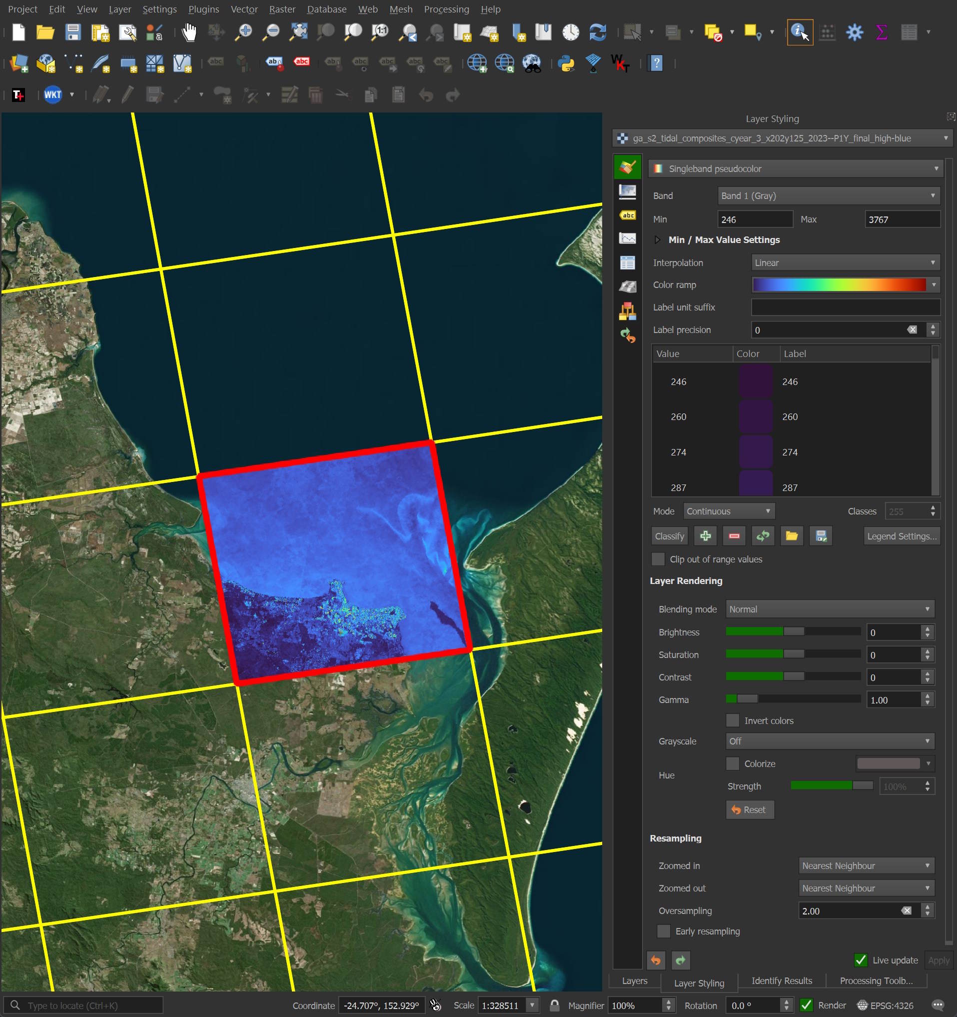
Below is a single GeoTIFF rendered on the grid used for this dataset. It's using a rainbow colour ramp.
Multispectral Imagery
A single GeoTIFF can be 10 - 15 MB and will represent one of the many bands supported by Sentinel-2. Below are the number of GeoTIFFs broken down by band and year.
WITH a AS (
    SELECT   band,
             year,
             COUNT(DISTINCT Key) AS num_keys
    FROM     s3
    WHERE    format = 'tif'
    GROUP BY 1, 2
)
PIVOT    a
ON       year
USING    SUM(num_keys)
GROUP BY band
ORDER BY band;
┌─────────────────┬────────┬────────┬────────┬────────┬────────┬────────┬────────┬────────┐
│      band       │  2016  │  2017  │  2018  │  2019  │  2020  │  2021  │  2022  │  2023  │
│     varchar     │ int128 │ int128 │ int128 │ int128 │ int128 │ int128 │ int128 │ int128 │
├─────────────────┼────────┼────────┼────────┼────────┼────────┼────────┼────────┼────────┤
│ blue            │   1940 │   2728 │   2722 │   2722 │   2722 │   2722 │   2722 │   2712 │
│ coastal-aerosol │   1940 │   2728 │   2722 │   2722 │   2722 │   2722 │   2722 │   2712 │
│ green           │   1940 │   2728 │   2722 │   2722 │   2722 │   2722 │   2722 │   2712 │
│ nir-1           │   1940 │   2728 │   2722 │   2722 │   2722 │   2722 │   2722 │   2712 │
│ nir-2           │   1940 │   2728 │   2722 │   2722 │   2722 │   2722 │   2722 │   2712 │
│ red             │   1940 │   2728 │   2722 │   2722 │   2722 │   2722 │   2722 │   2712 │
│ red-edge-1      │   1940 │   2728 │   2722 │   2722 │   2722 │   2722 │   2722 │   2712 │
│ red-edge-2      │   1940 │   2728 │   2722 │   2722 │   2722 │   2722 │   2722 │   2712 │
│ red-edge-3      │   1940 │   2728 │   2722 │   2722 │   2722 │   2722 │   2722 │   2712 │
│ swir-2          │   1940 │   2728 │   2722 │   2722 │   2722 │   2722 │   2722 │   2712 │
│ swir-3          │   1940 │   2728 │   2722 │   2722 │   2722 │   2722 │   2722 │   2712 │
├─────────────────┴────────┴────────┴────────┴────────┴────────┴────────┴────────┴────────┤
│ 11 rows                                                                       9 columns │
└─────────────────────────────────────────────────────────────────────────────────────────┘
The GeoTIFFs are compressed using DEFLATE.
$ gdalinfo \
    -json \
    ga_s2_tidal_composites_cyear_3_x202y125_2023--P1Y_final_high-blue.tif \
    | jq -S '.metadata'
{
  "": {
    "AREA_OR_POINT": "Area"
  },
  "IMAGE_STRUCTURE": {
    "COMPRESSION": "DEFLATE",
    "INTERLEAVE": "BAND",
    "LAYOUT": "COG",
    "PREDICTOR": "2"
  }
}
This means imagery over open ocean will often compress better than imagery captured over land.
Below I'll download the grid system used by this dataset.
$ wget -c https://data.dea.ga.gov.au/derivative/ga_summary_grid_sentinel_c3.geojson
I'll then build a heatmap showing how many MBs of GeoTIFFs have been collected for each tile.
$ ~/duckdb dea.duckdb
CREATE OR REPLACE TABLE grid AS
    SELECT geometry,
           ix AS x,
           iy AS y
    FROM (
        SELECT ST_GEOMFROMGEOJSON(a.geometry) AS geometry,
               UNNEST(a.properties)
        FROM (SELECT UNNEST(features) a
              FROM   READ_JSON('ga_summary_grid_sentinel_c3.geojson')));

COPY (
    SELECT   ROUND(SUM(a.Size) / 1024 ** 2)::INT AS MB,
             ST_ASWKB(b.geometry) geometry
    FROM     s3 a
    JOIN     grid b ON a.x = b.x AND a.y = b.y
    WHERE    format = 'tif'
    GROUP BY 2
) TO 'grid_stats.gpkg'
  WITH (FORMAT GDAL,
        DRIVER 'GPKG',
        LAYER_CREATION_OPTIONS 'WRITE_BBOX=YES');
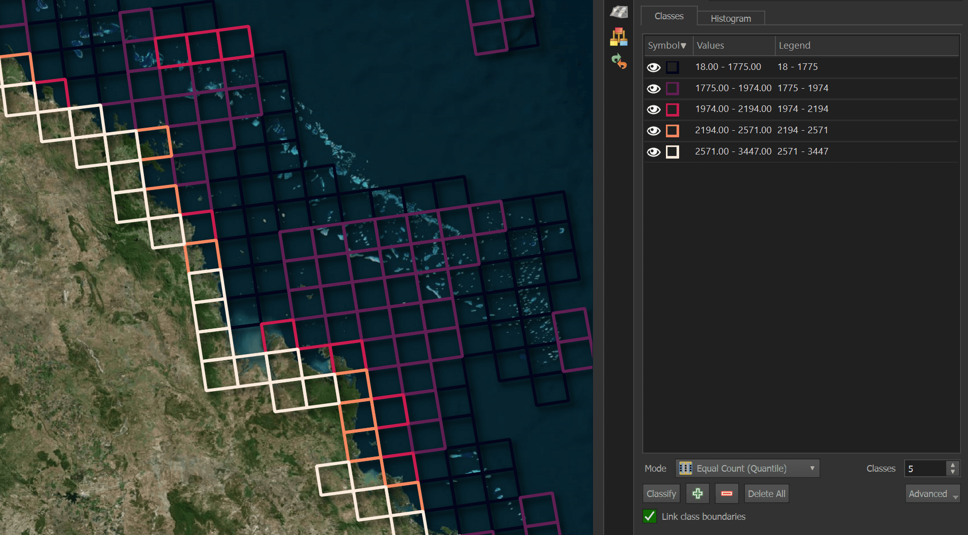
Below you can see the lighter tiles have ~2.5 - 3.4 GB of GeoTIFFs while the darker tiles have less than 1.8 GB.
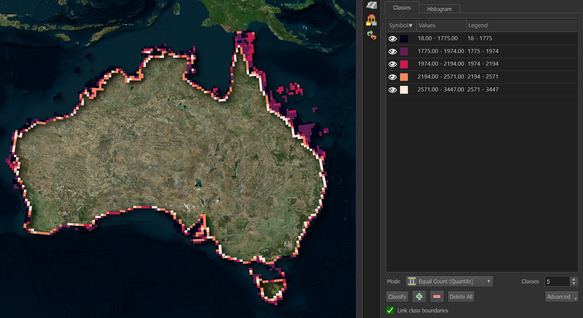
Along Queensland's coastline you can see the divide between imagery taken over land and the ocean.
With the exception of 2016, any given band has ~26 - 35 GB worth of GeoTIFFs for any given year.
WITH a AS (
    FROM  s3
    WHERE format = 'tif'
)
PIVOT    a
ON       year
USING    CEIL(SUM(Size) / 1024 ** 3)::INT
GROUP BY band
ORDER BY band;
┌─────────────────┬───────┬───────┬───────┬───────┬───────┬───────┬───────┬───────┐
│      band       │ 2016  │ 2017  │ 2018  │ 2019  │ 2020  │ 2021  │ 2022  │ 2023  │
│     varchar     │ int32 │ int32 │ int32 │ int32 │ int32 │ int32 │ int32 │ int32 │
├─────────────────┼───────┼───────┼───────┼───────┼───────┼───────┼───────┼───────┤
│ blue            │    24 │    34 │    34 │    33 │    34 │    34 │    33 │    33 │
│ coastal-aerosol │    19 │    27 │    26 │    26 │    26 │    26 │    26 │    26 │
│ green           │    25 │    34 │    34 │    34 │    34 │    34 │    34 │    34 │
│ nir-1           │    25 │    36 │    35 │    35 │    35 │    35 │    35 │    35 │
│ nir-2           │    23 │    33 │    32 │    32 │    32 │    32 │    32 │    32 │
│ red             │    25 │    35 │    34 │    34 │    34 │    34 │    34 │    34 │
│ red-edge-1      │    22 │    31 │    31 │    31 │    31 │    31 │    31 │    31 │
│ red-edge-2      │    23 │    32 │    32 │    32 │    32 │    32 │    32 │    32 │
│ red-edge-3      │    23 │    32 │    32 │    32 │    32 │    32 │    32 │    32 │
│ swir-2          │    22 │    31 │    31 │    31 │    31 │    31 │    31 │    31 │
│ swir-3          │    22 │    30 │    30 │    30 │    30 │    30 │    30 │    30 │
├─────────────────┴───────┴───────┴───────┴───────┴───────┴───────┴───────┴───────┤
│ 11 rows                                                               9 columns │
└─────────────────────────────────────────────────────────────────────────────────┘
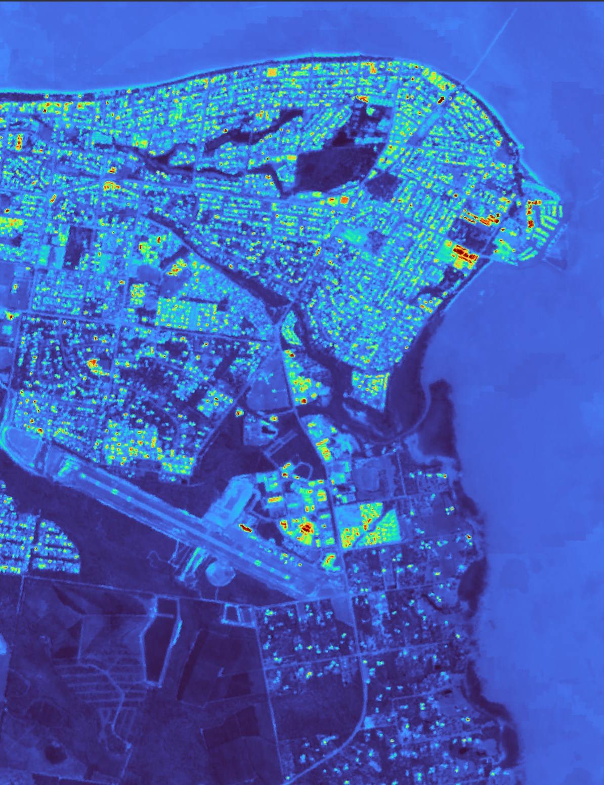
Urban Imagery
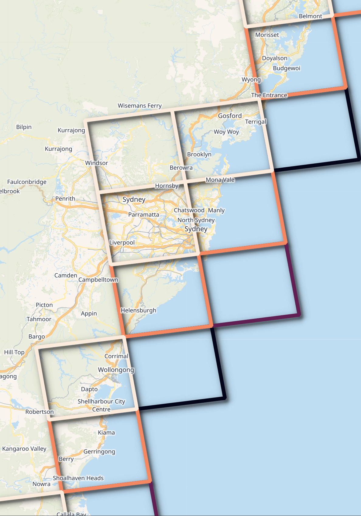
Imagery can often but not always fully cover Australia's coastal population centres. Below much of Sydney has imagery but the settlements further west aren't covered by this dataset.
The following used OpenStreetMap's (OSM) vector basemap.
Awesome Spectral Indices
The Awesome Spectral Indices project lists hundreds of chemical and naturally-occurring phenomenon that can be detected from multi- and hyperspectral imagery.

The bands in the GeoTIFFs can be paired with known algorithms that can identify things that are either invisible to the naked eye or hard to confirm with RGB-based analysis alone.
Below are a few of the soil-specific indices listed in the project. Signatures that are compatible with Sentinel-2 are tagged as such.
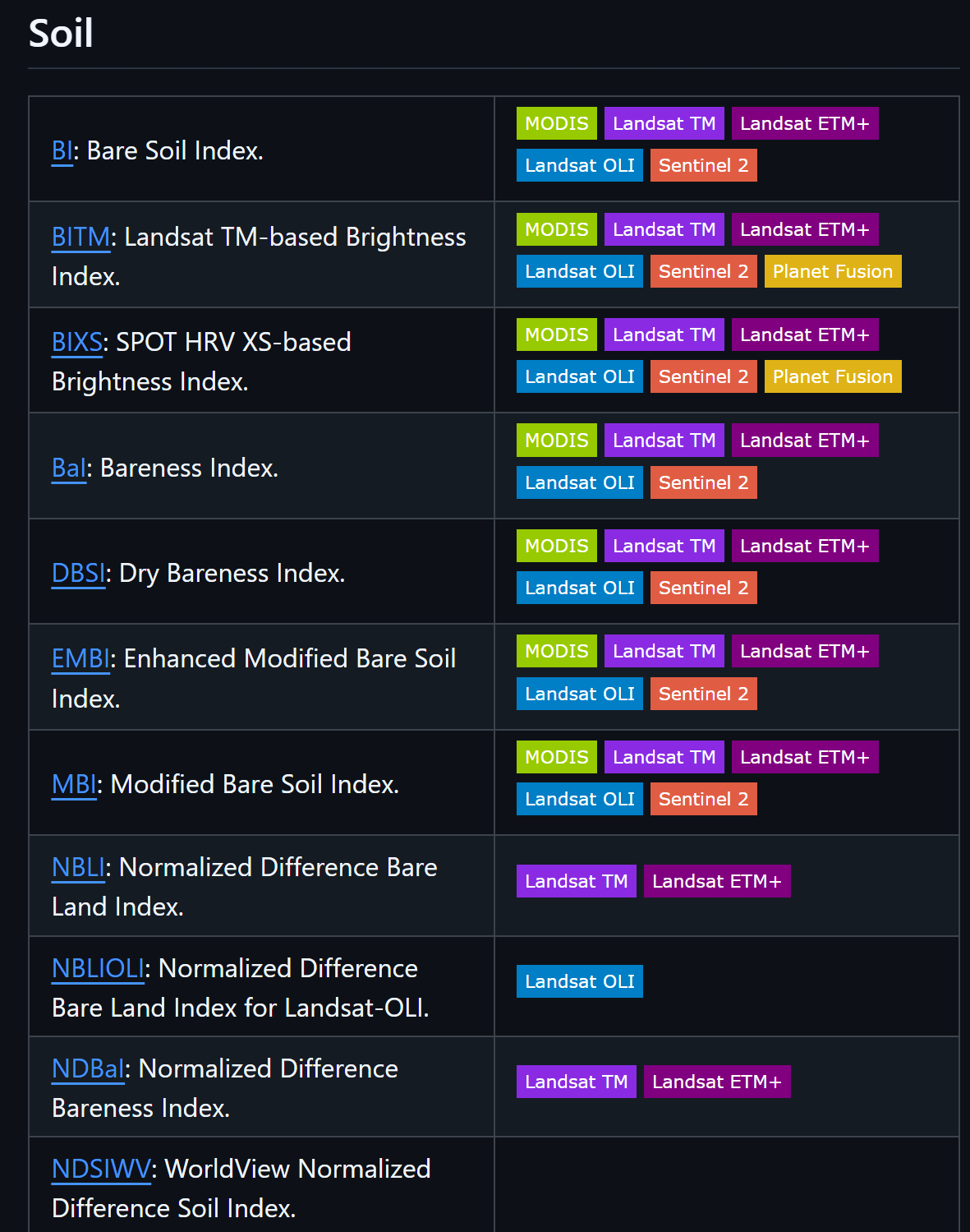
There is a package called spyndex which provides Python bindings for the Awesome Spectral Indices project as well.
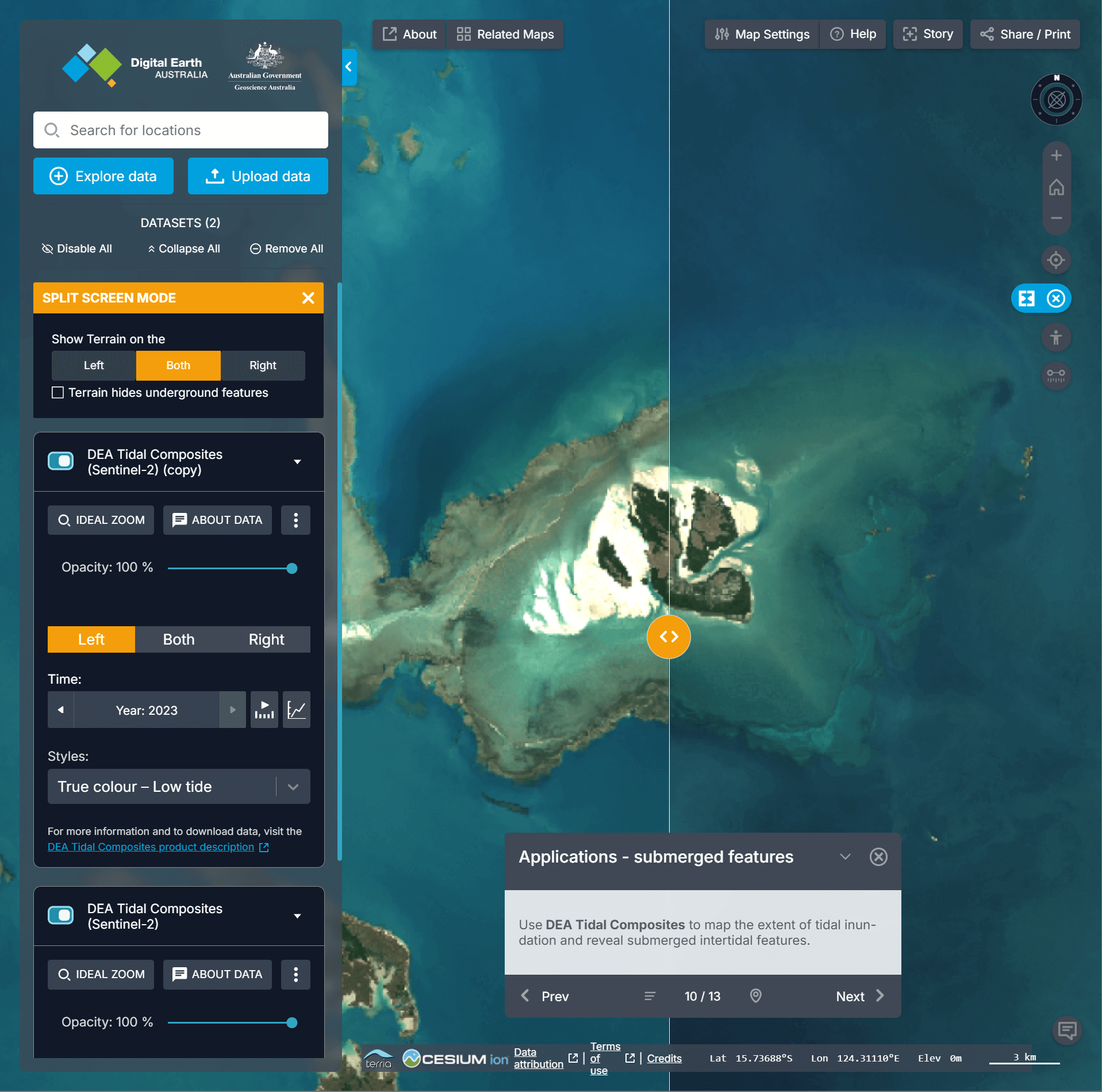
Web Viewer
The Tidal Composites dataset also has a web viewer set up.
Below is a screenshot demonstrating false-colour tidal composites where a slider can compare data between different years.
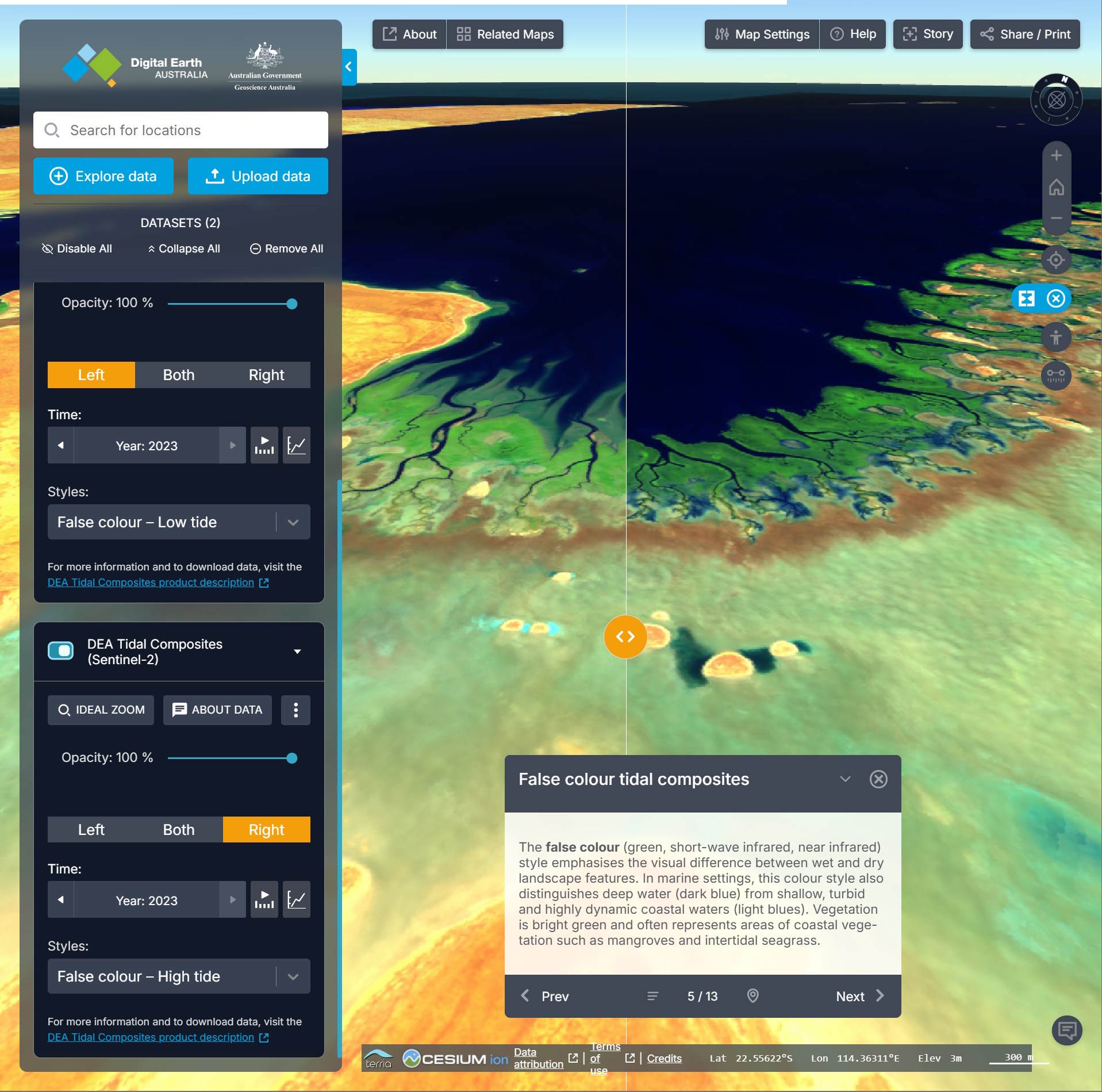
Below low tide lines are being compared between two different years.