Umbra Space is a 9-year-old manufacturer and operator of a Synthetic Aperture Radar (SAR) satellite fleet. These satellites can see through clouds, smoke, rain, snow and certain types of camouflage attempting to cover the ground below. SAR can capture images day or night at resolutions as fine as 16cm. SpaceX launched Umbra's first satellite in 2021 and has a total of ten in orbit at the moment.
SAR collects images via radar waves rather than optically. The resolution of the resulting imagery can be improved the longer a point is captured as the satellite flies over the Earth. This also means video is possible as shown with this SAR imagery from another provider below.

Umbra has an open data programme where they share SAR imagery from 500+ locations around the world. The points on the map below are coloured based on the satellite that captured the imagery.
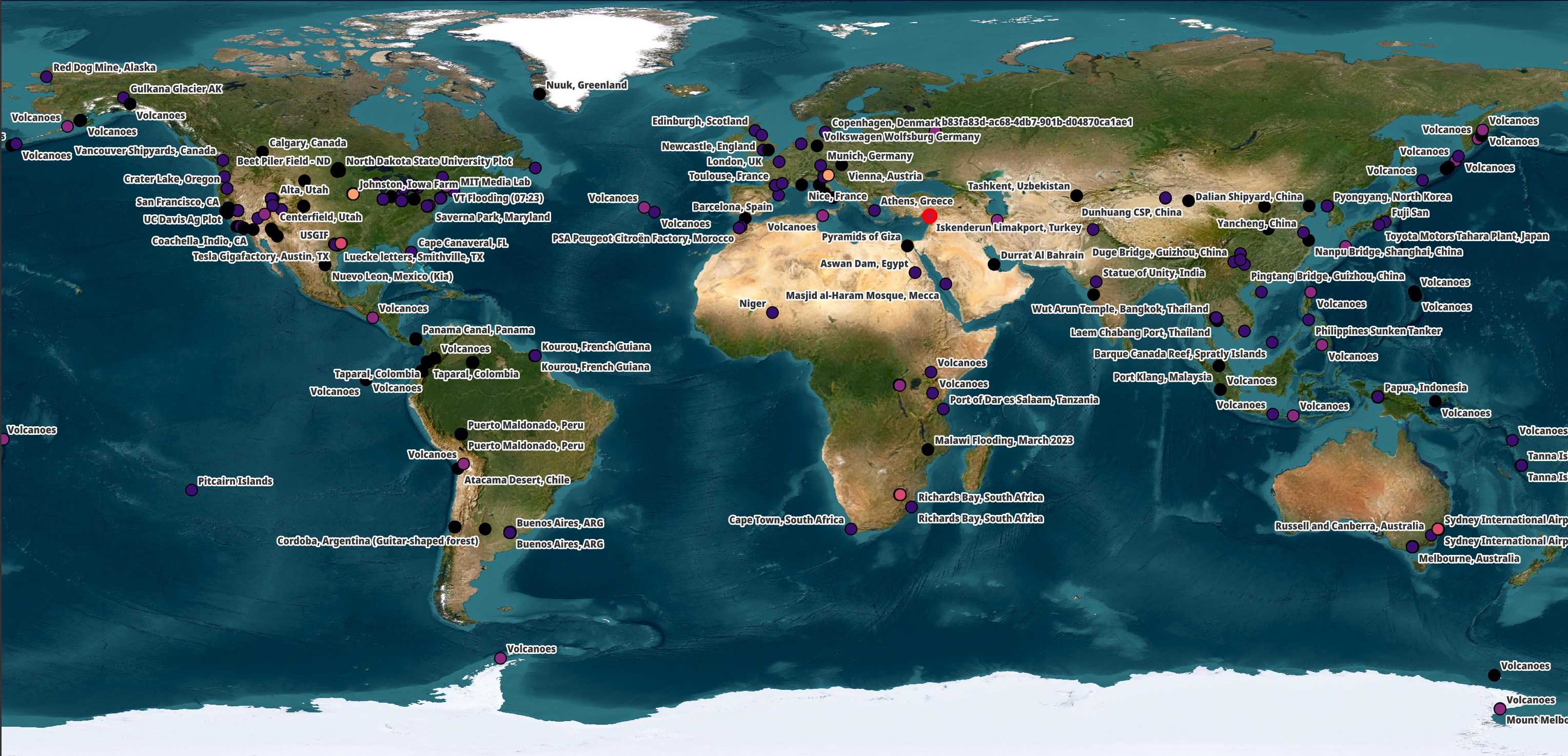
The subject matter largely focuses on manufacturing plants, airports, spaceports, large infrastructure projects and volcanos. Umbra state that the imagery being offered for free in their open data programme would have otherwise cost $4M to purchase.
Included in this feed are 140+ images of Bangkok Airport (BKK) that have been taken over the past two years. The image below links to the video I posted on LinkedIn.
Aircraft in SAR Imagery
Aircraft at known airports transmitting ADS-B messages do a good job of telling the world where they are. Paying ~$5K for this sort of SAR imagery doesn't make a lot of sense. But aircraft that have turned their ADS-B transponders off and are parked on a public highway are a different matter.
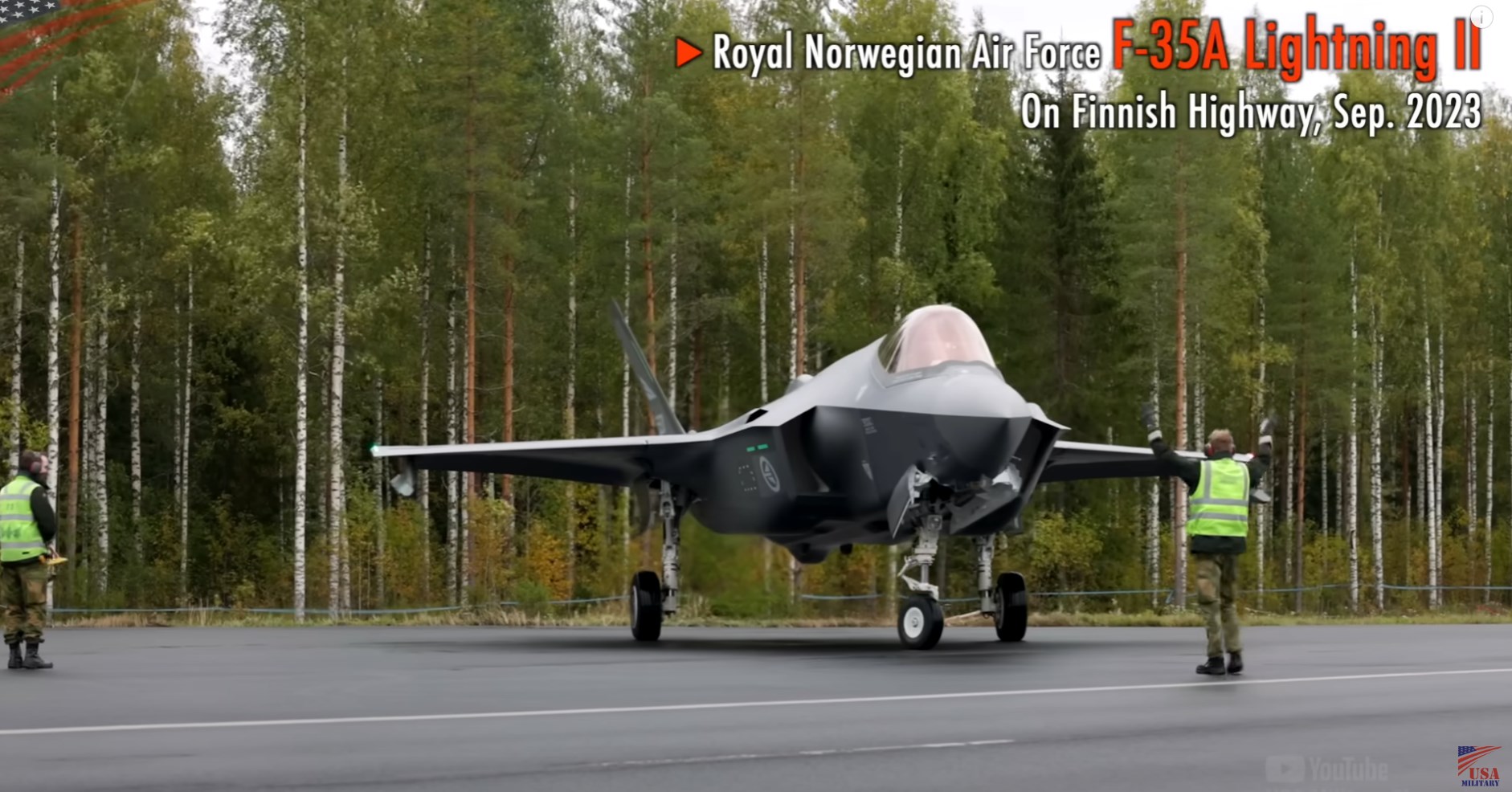
To add to this, it's rare in Northern Europe to have a clear sky regardless of the time of year. Clouds can be a real challenge here.
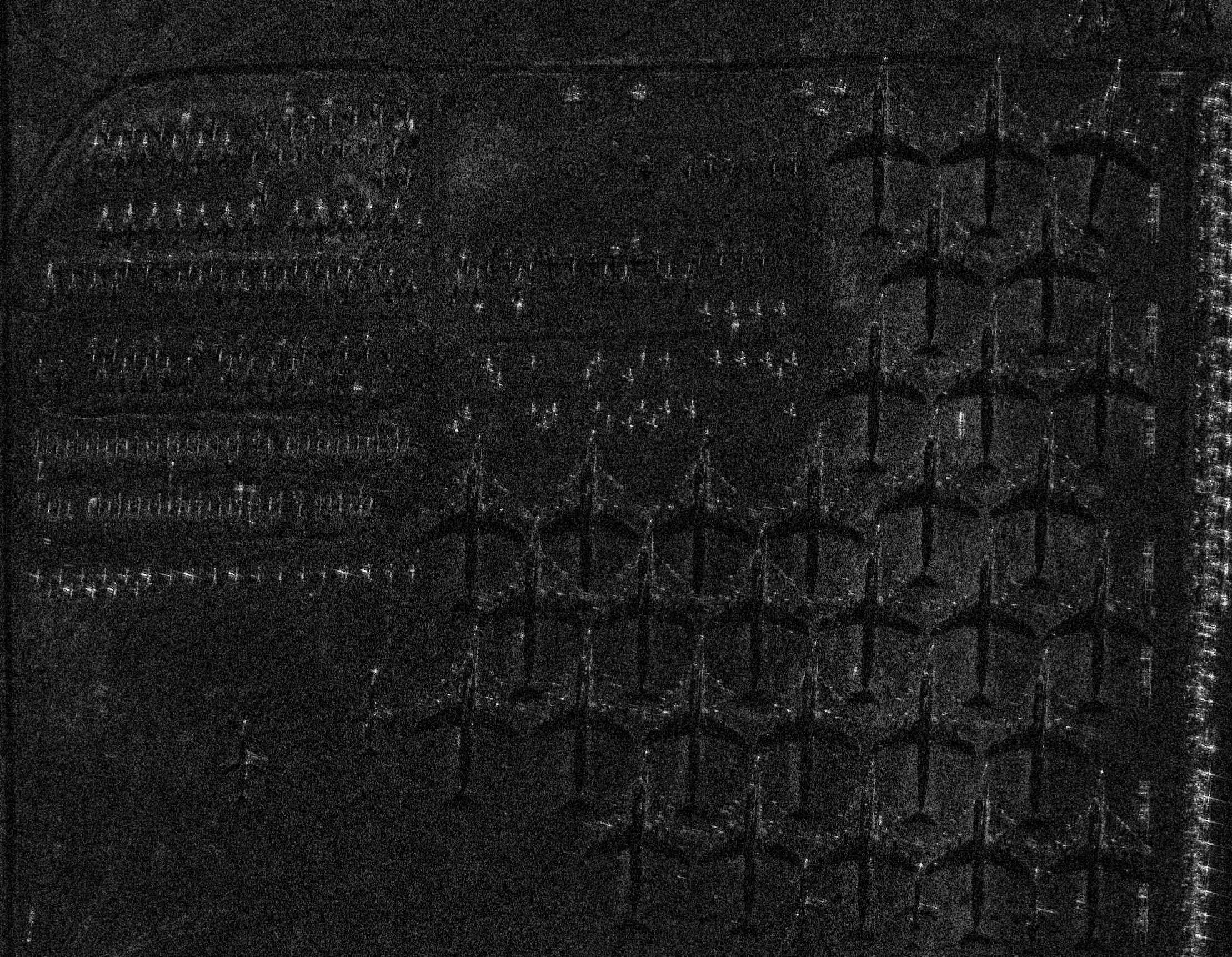
That said, some aircraft can be difficult to spot in SAR imagery. Below is Esri's satellite image of an Aircraft Boneyard.
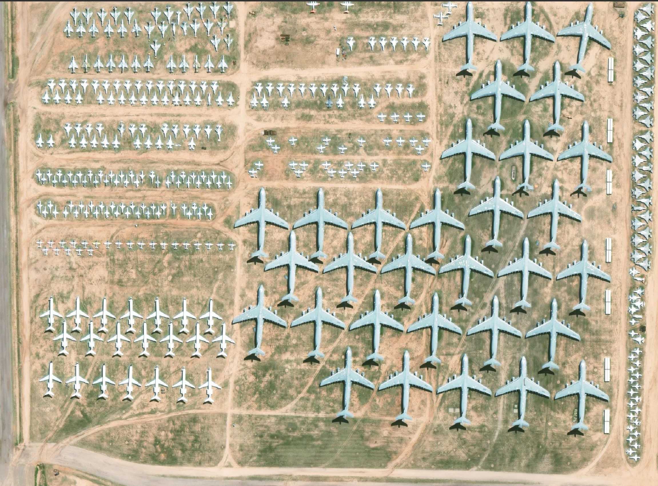
Below is Umbra's image of the same location. Though it was taken on a different day and some aircraft might have been moved around, you can see that a lot of the aircraft in the bottom left are barely visible unless you zoom in very closely and pay attention to artefacts that give away a large man-made object is present.
SARDet-100K & MSFA
In March, a paper was published titled "SARDet-100K: Towards Open-Source Benchmark and ToolKit for Large-Scale SAR Object Detection". It describes a new dataset called SARDet-100K and the Multi-Stage with Filter Augmentation (MSFA) framework for detecting objects in SAR imagery.
The dataset is made up of 117K SAR images with 246K objects annotated within them. These were sourced from ten existing datasets. The annotations highlight aircraft, bridges, cars, harbours, ships and tanks.
The framework tries to bridge the gap between RGB and SAR imagery. There are also several tools to help reduce multiplicative speckle noise and artefacts in SAR imagery.
In this post, I'll try to detect aircraft in Umbra's imagery using SARDet-100K and MSFA.
My Workstation
I'm using a 6 GHz Intel Core i9-14900K CPU. It has 8 performance cores and 16 efficiency cores with a total of 32 threads and 32 MB of L2 cache. It has a liquid cooler attached and is housed in a spacious, full-sized, Cooler Master HAF 700 computer case. I've come across videos on YouTube where people have managed to overclock the i9-14900KF to 9.1 GHz.
The system has 96 GB of DDR5 RAM clocked at 6,000 MT/s and a 5th-generation, Crucial T700 4 TB NVMe M.2 SSD which can read at speeds up to 12,400 MB/s. There is a heatsink on the SSD to help keep its temperature down. This is my system's C drive.
The system is powered by a 1,200-watt, fully modular, Corsair Power Supply and is sat on an ASRock Z790 Pro RS Motherboard.
I'm running Ubuntu 22 LTS via Microsoft's Ubuntu for Windows on Windows 11 Pro. In case you're wondering why I don't run a Linux-based desktop as my primary work environment, I'm still using an Nvidia GTX 1080 GPU which has better driver support on Windows and I use ArcGIS Pro from time to time which only supports Windows natively.
Installing Prerequisites
I'll be using Python and a few other tools to help analyse the data in this post.
$ sudo apt update
$ sudo apt install \
    aws-cli \
    gdal-bin \
    jq \
    python3-pip \
    python3-virtualenv
I'll set up a Python Virtual Environment and install some dependencies.
$ virtualenv ~/.msfa
$ source ~/.msfa/bin/activate

$ pip install \
    boto3 \
    geopandas \
    osgeo \
    pandas \
    rich \
    shapely \
    typer
The following will install some PyTorch dependencies.
$ pip install \
    torch==2.0.1 \
    torchvision==0.15.2 \
    torchaudio==2.0.2 \
    --index-url https://download.pytorch.org/whl/cu118
MSFA relies on a number of OpenMMLab packages.
$ pip install -U openmim
$ mim install -U \
    mmengine \
    mmcv \
    mmdet \
    mmpretrain
The following will install the MSFA Framework.
$ git clone https://github.com/zcablii/SARDet_100K
$ cd SARDet_100K/MSFA

$ pip install -r requirements.txt
$ pip install -v -e .
I had some issues with SciPy 1.14.1 so I've downgraded to version 1.12.0.
$ pip install -U 'scipy<1.13'
I'll use DuckDB, along with its H3, JSON, Parquet and Spatial extensions, in this post.
$ cd ~
$ wget -c https://github.com/duckdb/duckdb/releases/download/v1.0.0/duckdb_cli-linux-amd64.zip
$ unzip -j duckdb_cli-linux-amd64.zip
$ chmod +x duckdb
$ ~/duckdb
INSTALL h3 FROM community;
INSTALL json;
INSTALL parquet;
INSTALL spatial;
I'll set up DuckDB to load every installed extension each time it launches.
$ vi ~/.duckdbrc
.timer on
.width 180
LOAD h3;
LOAD json;
LOAD parquet;
LOAD spatial;
The maps in this post were rendered with QGIS version 3.38.0. QGIS is a desktop application that runs on Windows, macOS and Linux. The application has grown in popularity in recent years and has ~15M application launches from users around the world each month.
I used QGIS' Tile+ plugin to add geospatial context with Esri's World Imagery and CARTO's Basemaps to the maps.
Downloading Satellite Imagery
Umbra's Open Data feed has grown to just under 45 TB as of this writing.
$ mkdir -p ~/umbra_bkk
$ cd ~/umbra_bkk

$ aws --no-sign-request \
      --output json \
      s3api \
      list-objects \
      --bucket umbra-open-data-catalog \
      --max-items=1000000 \
    | jq -c '.Contents[]' \
    > umbra.s3.json
$ echo "Total objects: " `wc -l umbra.s3.json | cut -d' ' -f1`, \
   " TB: " `jq .Size umbra.s3.json | awk '{s+=$1}END{print s/1024/1024/1024/1024}'`
Total objects: 33813, TB: 44.9067
I'll download the GeoTIFF deliverables and JSON Metadata files for Bangkok Airport. These add up to ~35 GB in size.
$ for FORMAT in json tif; do
    aws s3 --no-sign-request \
           sync \
           --exclude="*" \
           --include="*.$FORMAT" \
           "s3://umbra-open-data-catalog/sar-data/tasks/Suvarnabhumi International Airport, Thailand/" \
           ~/umbra_bkk/
  done
Umbra's Bangkok Airport Imagery
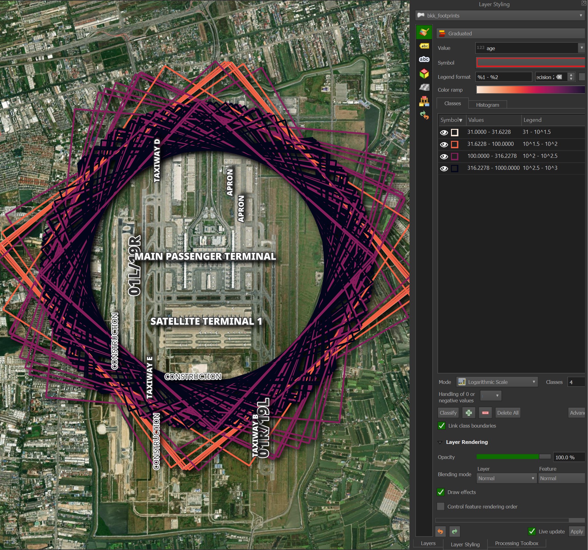
The 140+ images taken of BKK airport all have a footprint 5 x 5KM. That said, the footprints all cover slightly different areas. Below is a rendering of the footprints over the two year period.
I'll extract some metadata of interest and load it into a DuckDB table.
$ cd ~/umbra_bkk
$ python3
import json
from   pathlib       import Path

from   rich.progress import track


with open('enriched.json', 'w') as f:
    for filename in track(list(Path('.').glob('**/*_METADATA.json'))):
        rec = json.loads(open(filename, 'r').read())

        out = {'filename':       str(filename),
               'sat_num':        rec['umbraSatelliteName'],
               'imaging_mode':   rec['imagingMode'],
               'polarisation':   ', '.join(sorted(rec['collects'][0]['polarizations'])),
               'start':          rec['collects'][0]['startAtUTC'],
               'finish':         rec['collects'][0]['endAtUTC'],
               'radarBand':      rec['collects'][0]['radarBand'],
               'azimuth_meters': rec['collects'][0]['maxGroundResolution']['azimuthMeters'],
               'range_meters':   rec['collects'][0]['maxGroundResolution']['rangeMeters'],
               'azimuth_looks':  rec['derivedProducts']['GEC'][0]['looks']['azimuth'],
               'range_looks':    rec['derivedProducts']['GEC'][0]['looks']['range']}

        f.write(json.dumps(out, sort_keys=True) + '\n')
$ ~/duckdb
CREATE OR REPLACE TABLE umbra AS
    SELECT * EXCLUDE(start, finish),
           start::DATETIME AS start,
           finish::DATETIME AS finish
    FROM   READ_JSON('enriched.json');
Below are the number of images for each month and the satellite that took them.
WITH a AS (
    SELECT STRFTIME(start, '%Y-%m') yyyy_mm,
           sat_num,
           count(*) num_recs
    FROM umbra
    GROUP BY 1, 2
    ORDER BY 1, 2
)
PIVOT    a
ON       sat_num
USING    SUM(num_recs)
GROUP BY yyyy_mm
ORDER BY yyyy_mm;
┌─────────┬──────────┬──────────┬──────────┬──────────┐
│ yyyy_mm │ UMBRA_04 │ UMBRA_05 │ UMBRA_06 │ UMBRA_08 │
│ varchar │  int128  │  int128  │  int128  │  int128  │
├─────────┼──────────┼──────────┼──────────┼──────────┤
│ 2023-02 │        7 │        5 │          │          │
│ 2023-03 │        6 │        5 │          │          │
│ 2023-04 │        8 │        7 │          │          │
│ 2023-05 │        5 │        6 │          │          │
│ 2023-06 │        3 │       10 │        6 │          │
│ 2023-07 │        4 │        7 │        2 │          │
│ 2023-08 │        6 │        8 │          │          │
│ 2023-09 │        4 │        3 │          │          │
│ 2023-10 │        3 │        4 │          │          │
│ 2023-11 │        4 │        2 │          │          │
│ 2024-01 │        1 │        3 │        4 │          │
│ 2024-02 │          │        3 │        6 │          │
│ 2024-03 │        2 │        1 │          │        1 │
│ 2024-05 │          │        1 │        2 │          │
│ 2024-06 │          │        1 │          │          │
│ 2024-07 │          │          │        1 │          │
│ 2024-08 │          │        1 │          │          │
├─────────┴──────────┴──────────┴──────────┴──────────┤
│ 17 rows                                   5 columns │
└─────────────────────────────────────────────────────┘
All of the images have the same polarisation and use the X radar band.
SELECT   imaging_mode,
         polarisation,
         radarBand,
         COUNT(*)
FROM     umbra
GROUP BY 1, 2, 3;
┌──────────────┬──────────────┬───────────┬──────────────┐
│ imaging_mode │ polarisation │ radarBand │ count_star() │
│   varchar    │   varchar    │  varchar  │    int64     │
├──────────────┼──────────────┼───────────┼──────────────┤
│ SPOTLIGHT    │ VV           │ X         │          142 │
└──────────────┴──────────────┴───────────┴──────────────┘
The highest resolution imagery in this dataset is 17.48 cm.
SELECT   sat_num,
         ROUND(MIN(azimuth_meters * 100), 2) AS cm_res,
FROM     umbra
GROUP BY 1
ORDER BY 2
┌──────────┬────────┐
│ sat_num  │ cm_res │
│ varchar  │ double │
├──────────┼────────┤
│ UMBRA_06 │  17.48 │
│ UMBRA_05 │  17.73 │
│ UMBRA_08 │   25.0 │
│ UMBRA_04 │   25.0 │
└──────────┴────────┘
Below are the resolution buckets for each satellite.
WITH a AS (
    SELECT (ROUND(ROUND(azimuth_meters * 100) / 10) * 10)::INT AS cm_res,
           sat_num
    FROM   umbra
)
PIVOT    a
ON       sat_num
USING    COUNT(*)
GROUP BY cm_res
ORDER BY cm_res;
┌────────┬──────────┬──────────┬──────────┬──────────┐
│ cm_res │ UMBRA_04 │ UMBRA_05 │ UMBRA_06 │ UMBRA_08 │
│ int32  │  int64   │  int64   │  int64   │  int64   │
├────────┼──────────┼──────────┼──────────┼──────────┤
│     20 │        0 │        4 │        6 │        0 │
│     30 │        2 │        5 │        7 │        1 │
│     40 │        8 │        8 │        4 │        0 │
│     50 │       34 │       36 │        1 │        0 │
│     60 │        7 │       13 │        3 │        0 │
│     70 │        2 │        1 │        0 │        0 │
└────────┴──────────┴──────────┴──────────┴──────────┘
The majority of imagery only had one look but there are a few 2 and 3-look images in this dataset as well.
SELECT   ROUND(azimuth_looks)::INT as looks,
         COUNT(*) num_images
FROM     umbra
GROUP BY 1
ORDER BY 1;
┌───────┬────────────┐
│ looks │ num_images │
│ int32 │   int64    │
├───────┼────────────┤
│     1 │        119 │
│     2 │         21 │
│     3 │          2 │
└───────┴────────────┘
The number of looks correlates with a higher resolution.
WITH a AS (
    SELECT (ROUND(ROUND(azimuth_meters * 100) / 10) * 10)::INT AS cm_res,
           ROUND(azimuth_looks)::INT AS looks
    FROM   umbra
)
PIVOT    a
ON       looks
USING    COUNT(*)
GROUP BY cm_res
ORDER BY cm_res;
┌────────┬───────┬───────┬───────┐
│ cm_res │   1   │   2   │   3   │
│ int32  │ int64 │ int64 │ int64 │
├────────┼───────┼───────┼───────┤
│     20 │     0 │     8 │     2 │
│     30 │     2 │    13 │     0 │
│     40 │    20 │     0 │     0 │
│     50 │    71 │     0 │     0 │
│     60 │    23 │     0 │     0 │
│     70 │     3 │     0 │     0 │
└────────┴───────┴───────┴───────┘
Downloading SARDet_100K Weights
SARDet_100K hosts their model weights on Baidu Disk and OneDrive. The ZIP file with the weights is 20 GB. Below are its contents.
$ du -hs /home/mark/ckpts/* \
    | grep '[0-9][MG]' \
    | cut -d/ -f1,5 \
    | sed 's/\///g'
1.1G    convnext_b_sar
1.1G    convnext_b_sar_wavelet
598M    convnext_s_sar
603M    convnext_s_sar_wavelet
339M    convnext_t_sar
344M    convnext_t_sar_wavelet
457M    fg_frcnn_dota_pretrain_sar_convnext_b_wavelet
228M    fg_frcnn_dota_pretrain_sar_convnext_t_wavelet
287M    fg_frcnn_dota_pretrain_sar_r101_wavelet
346M    fg_frcnn_dota_pretrain_sar_r152_wavelet
308M    fg_frcnn_dota_pretrain_sar_swin_s_wavelet
227M    fg_frcnn_dota_pretrain_sar_swin_t_wavelet
222M    fg_frcnn_dota_pretrain_sar_van_b_wavelet
173M    fg_frcnn_dota_pretrain_sar_van_s_wavelet
135M    fg_frcnn_dota_pretrain_sar_van_t_wavelet
214M    fg_frcnn_dota_pretrain_sar_wavelet_r50
2.2G    gfl_r50_denodet_sardet
210M    hrsid_frcnn_van_sar_wavelet_bs32_3
481M    pretrain_frcnn_dota_convnext_b_sar_wavelet
335M    pretrain_frcnn_dota_convnext_s_sar_wavelet
2.3G    pretrain_frcnn_dota_r101_sar
312M    pretrain_frcnn_dota_r101_sar_wavelet
372M    pretrain_frcnn_dota_r152_sar_wavelet
239M    pretrain_frcnn_dota_r50_sar_wavelet
333M    pretrain_frcnn_dota_swin_s_sar_wavelet
251M    pretrain_frcnn_dota_swin_t_sar_wavelet
246M    pretrain_frcnn_dota_van_b_sar_wavelet
197M    pretrain_frcnn_dota_van_s_sar_wavelet
160M    pretrain_frcnn_dota_van_t_sar_wavelet
377M    r101_sar_epoch_100.pth
382M    r101_sar_wavelet_epoch_100.pth
502M    r152_sar_wavelet
231M    r50_sar_epoch_100.pth
237M    r50_sar_wavelet_epoch_100.pth
210M    ssdd_frcnn_van_sar_wavelet_bs32_3
1.1G    swin_b_sar
596M    swin_s_sar
601M    swin_s_sar_wavelet
351M    swin_t_sar
356M    swin_t_sar_wavelet
338M    van_b_sar_wavelet_epoch_100.pth
173M    van_s_sar_epoch_100.pth
179M    van_s_sar_wavelet_epoch_100.pth
61M     van_t_sar_epoch_100.pth
66M     van_t_sar_wavelet_epoch_100.pth
SAR Aircraft Training Data
Three of the ten datasets in SARDet_100K contain aircraft imagery.
Datasets       | Objects     | Resolution | Band    | Polarization    | Satellites
---------------|-------------|------------|---------|-----------------|------------------------------
MSAR           | A, T, B, S  | ≤ 1m       | C       | HH, HV, VH, VV  | HISEA-1
SADD           | A           | 0.5-3m     | X       | HH              | TerraSAR-X
SAR-AIRcraft   | A           | 1m         | C       | Uni-polar       | GF-3
AIR_SARShip    | S           | 1,3m       | C       | VV              | GF-3
HRSID          | S           | 0.5-3m     | C/X     | HH, HV, VH, VV  | S-1B, TerraSAR-X, TanDEMX
ShipDataset    | S           | 3-25m      | C       | HH, VV, VH, HV  | S-1, GF-3
SSDD           | S           | 1-15m      | C/X     | HH, VV, VH, HV  | S-1, RadarSat-2, TerraSAR-X
OGSOD          | B, H, T     | 3m         | C       | VV/VH           | GF-3
SIVED          | C           | 0.1,0.3m   | Ka,Ku,X | VV/HH           | Airborne SAR synthetic slice
The object acronyms are (A)ircraft, (B)ridges, (C)ars, (H)arbours, (S)hips and (T)anks.
The Umbra imagery in this post uses VV polarisation which some of the MSAR data used as well.
SAR radar beams can switch between horizontal and vertical polarisation both when sending and receiving. These are denoted by two letters. For example: HV would mean horizontal transmission and vertical receiving.
Horizontal polarisation is ideal for flat and low surfaces, like rivers, bridges and power lines. Vertical polarisation is ideal for buildings, rough seas and transmission towers.
The aircraft training imagery was collected using the X band in some cases but the C band in others. The X band is good for urban monitoring and seeing through snow but it can't penetrate vegetation very well. This might make aircraft under a natural canopy harder to detect. The Umbra imagery in this post was all collected with the X band.
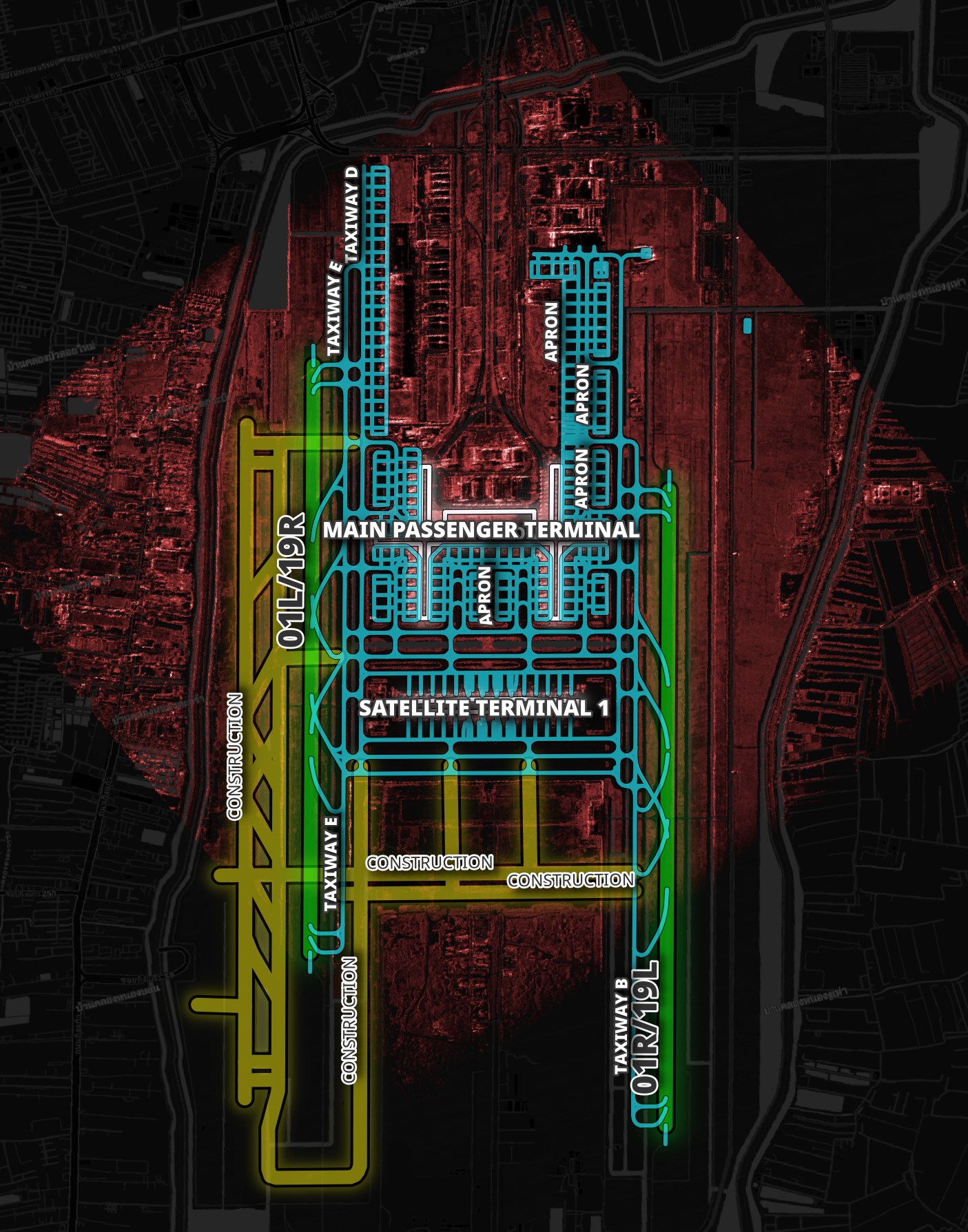
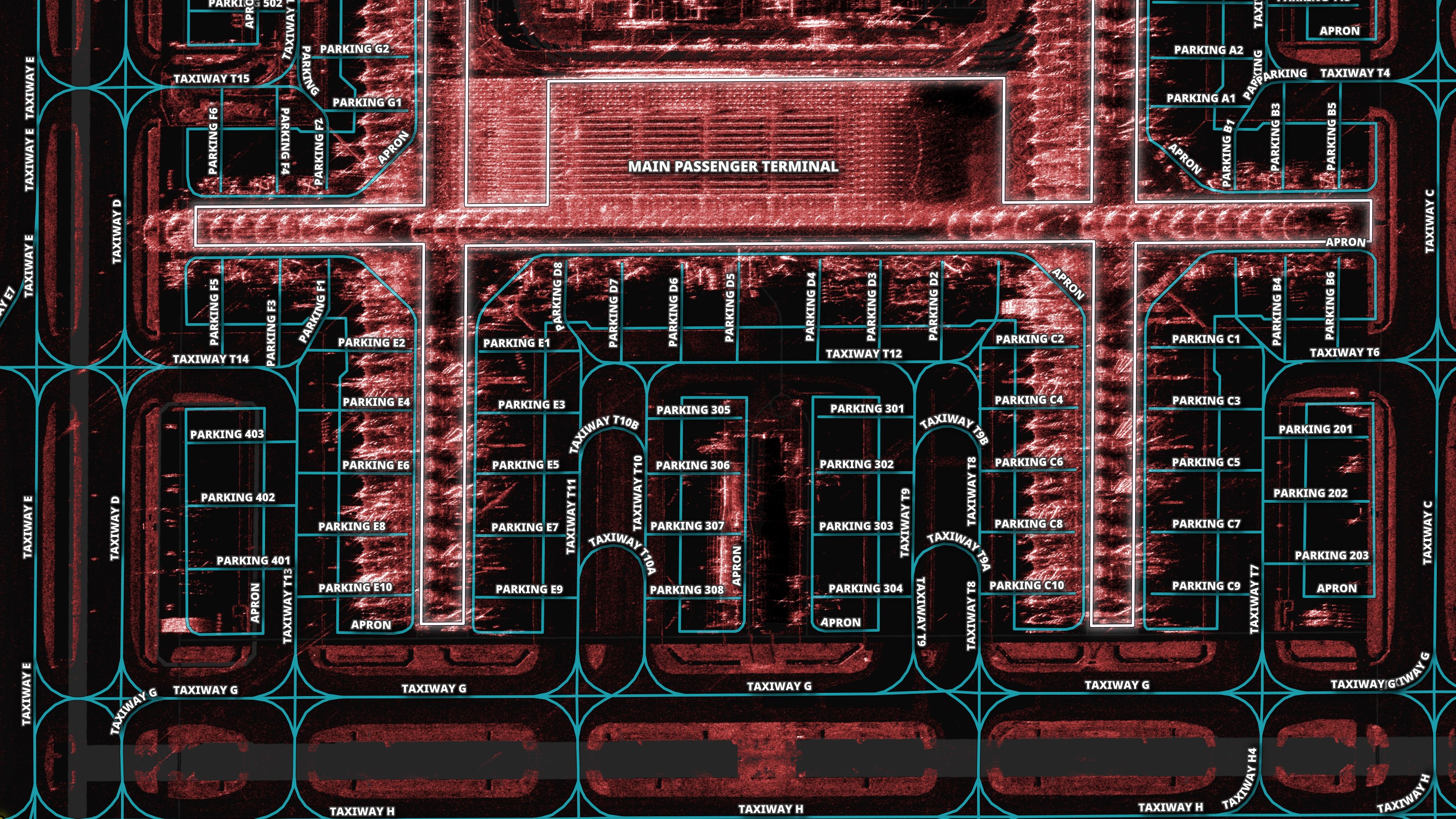
Bangkok Suvarnabhumi International Airport
I'll walk through the layout of Bangkok Suvarnabhumi International Airport (BKK). I used GeoFabrik's OpenStreetMap (OSM) distributable for Thailand and osm_split to extract the geometry and metadata in the following images.
There are aircraft parking gates south of the main passenger terminal and all around the satellite terminal.
Below is a closer view of the parking spots around the main passenger terminal.
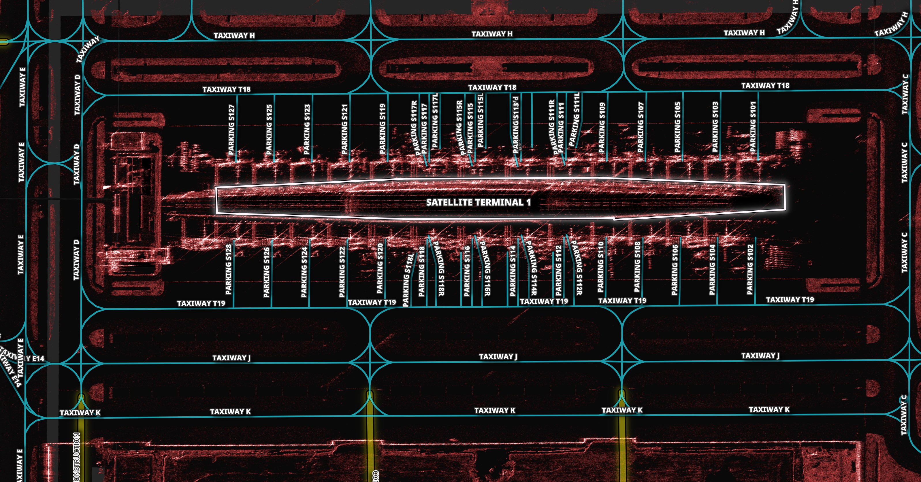
Below is a closer view of the parking spots around the satellite terminal.
I've overlaid four hours of ADS-B data from the evening of May 25th on the map. This gives a bit of ground truth as to where aircraft were located around the time Umbra took their image for that day.
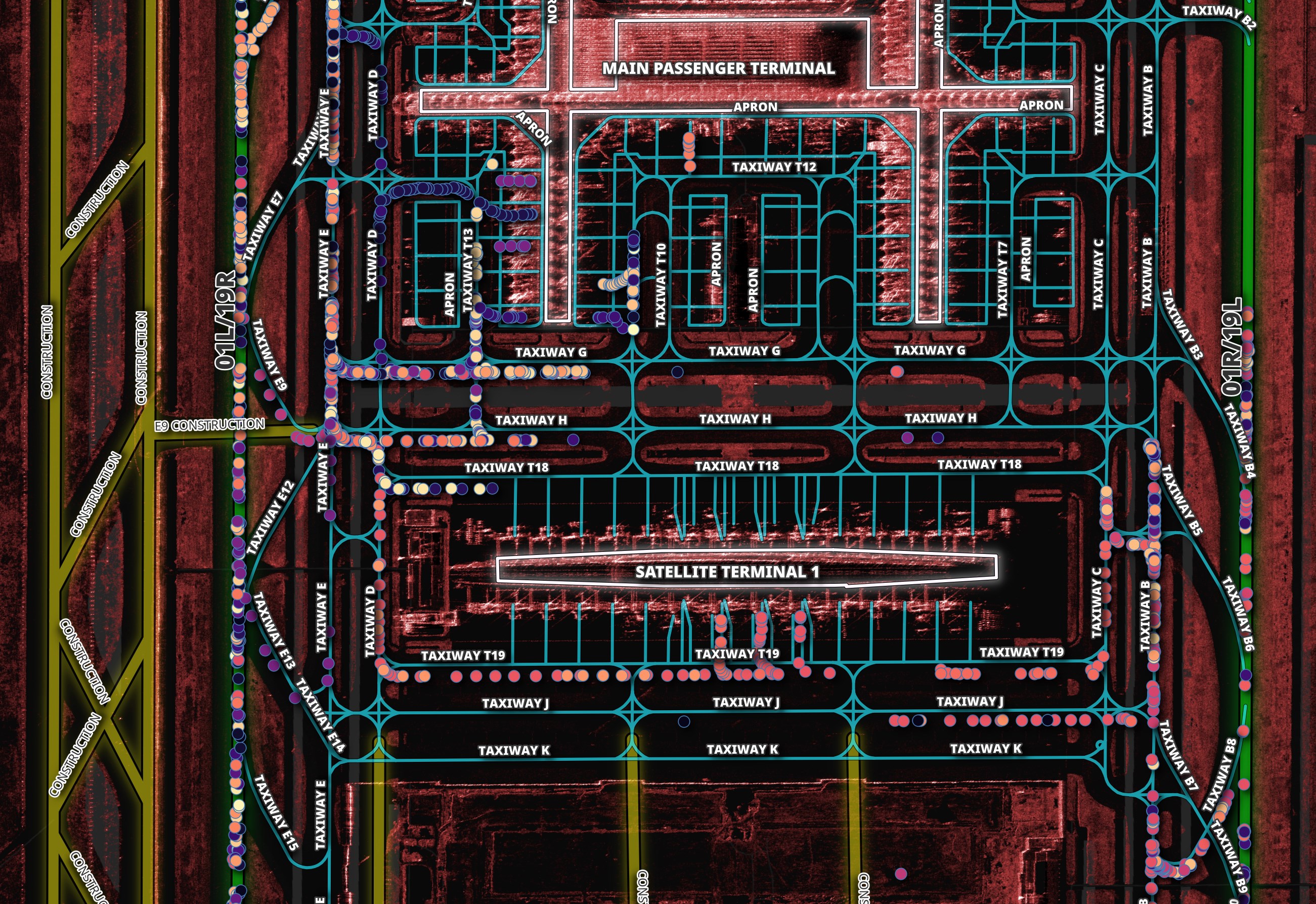
The ADS-B data was sourced from the adsb.lol project. I built a tool called adsb_json that converts the JSON adsb.lol produces into GeoPackage (GPKG) files.
DeonDet
I'll run DeonDet on Umbra's image of BKK for May 25th. Below is a configuration file that ships with MSFA.
$ cat ~/SARDet_100K/MSFA/local_configs/DeonDet/gfl_r50_denodet_sardet.py
_base_ = [
    '../../configs/_base_/datasets/SARDet_100k.py',
    '../../configs/_base_/schedules/schedule_1x.py', '../../configs/_base_/default_runtime.py'
]
num_classes = 6
model = dict(
    type='GFL',
    data_preprocessor=dict(
        type='DetDataPreprocessor',
        mean=[123.675, 116.28, 103.53],
        std=[58.395, 57.12, 57.375],
        bgr_to_rgb=True,
        pad_size_divisor=32),
    backbone=dict(
        type='ResNet',
        depth=50,
        num_stages=4,
        out_indices=(0, 1, 2, 3),
        frozen_stages=1,
        norm_cfg=dict(type='BN', requires_grad=True),
        norm_eval=True,
        style='pytorch',
        init_cfg=dict(type='Pretrained', checkpoint='torchvision://resnet50')),
    neck=dict(
        type='FrequencySpatialFPN',
        in_channels=[256, 512, 1024, 2048],
        out_channels=256,
        start_level=1,
        add_extra_convs='on_input',
        num_outs=5,
        norm_cfg=dict(type='GN', num_groups=32, requires_grad=True)),
    bbox_head=dict(
        type='GFLHead',
        num_classes=num_classes,
        in_channels=256,
        stacked_convs=4,
        feat_channels=256,
        anchor_generator=dict(
            type='AnchorGenerator',
            ratios=[1.0],
            octave_base_scale=8,
            scales_per_octave=1,
            strides=[8, 16, 32, 64, 128]),
        loss_cls=dict(
            type='QualityFocalLoss',
            use_sigmoid=True,
            beta=2.0,
            loss_weight=1.0),
        loss_dfl=dict(type='DistributionFocalLoss', loss_weight=0.25),
        reg_max=16,
        loss_bbox=dict(type='GIoULoss', loss_weight=2.0)),
    # training and testing settings
    train_cfg=dict(
        assigner=dict(type='ATSSAssigner', topk=9),
        allowed_border=-1,
        pos_weight=-1,
        debug=False),
    test_cfg=dict(
        nms_pre=1000,
        min_bbox_size=0,
        score_thr=0.05,
        nms=dict(type='nms', iou_threshold=0.6),
        max_per_img=100))


backend_args = None
train_pipeline = [
    dict(type='LoadImageFromFile', backend_args=backend_args),
    dict(type='LoadAnnotations', with_bbox=True),
    dict(type='Resize', scale=(1024, 1024), keep_ratio=False),
    dict(type='RandomFlip', prob=0.5),
    dict(type='PackDetInputs')
]

test_pipeline = [
    dict(type='LoadImageFromFile', backend_args=backend_args),
    dict(type='Resize', scale=(1024, 1024), keep_ratio=False),
    # If you don't have a gt annotation, delete the pipeline
    dict(type='LoadAnnotations', with_bbox=True),
    dict(
        type='PackDetInputs',
        meta_keys=('img_id', 'img_path', 'ori_shape', 'img_shape',
                   'scale_factor'))
]

train_dataloader = dict(
    dataset=dict(
        pipeline=train_pipeline))
val_dataloader = dict(
    dataset=dict(
        pipeline=test_pipeline))
test_dataloader = dict(
    dataset=dict(
        pipeline=test_pipeline))


# find_unused_parameters = True
optim_wrapper = dict(
    optimizer=dict(
        _delete_=True,
        betas=(
            0.9,
            0.999,
        ), lr=0.0001, type='AdamW', weight_decay=0.05),
    type='OptimWrapper')
I'll copy Umbra's image into a working folder.
$ mkdir ~/working
$ cd ~/working
$ cp ~/umbra_bkk/80f35b05-2902-46cc-9642-5d0e8916bf49/2024-05-25-15-37-54_UMBRA-06/2024-05-25-15-37-54_UMBRA-06_GEC.tif" ./
Rational Polynomial Coefficients
This year, Umbra began including Rational polynomial coefficient (RPC) metadata in their SAR imagery.
$ gdalinfo -json 2024-05-25-15-37-54_UMBRA-06_GEC.tif \
    | jq -S .metadata.RPC
{
  "ERR_BIAS": "-1",
  "ERR_RAND": "-1",
  "HEIGHT_OFF": "-30.6818097811395",
  "HEIGHT_SCALE": "1414.21349937642",
  "LAT_OFF": "13.6906792091218",
  "LAT_SCALE": "0.0138548308915265",
  "LINE_DEN_COEFF": "1 0 0 0 0 0 0 0 0 0 0 0 0 0 0 0 0 0 0 0",
  "LINE_NUM_COEFF": "1.02231794327927e-05 0.215896351104129 -0.481367152531649 -0.848789645419274 -1.03956610619756e-05 0.00802968239297444 -0.00163693193778641 9.08138917922306e-05 0.000110851333886418 -0.0101589838895881 2.87171326664789e-05 -9.52685642544797e-07 -1.04184901360726e-06 0.000306411120496931 1.41330069687536e-07 2.04421034231927e-07 -5.98024000515252e-05 -7.13359480585107e-05 -1.9284524777315e-07 -0.00026831462493207",
  "LINE_OFF": "8000",
  "LINE_SCALE": "9297.59735239297",
  "LONG_OFF": "100.750015998877",
  "LONG_SCALE": "0.0141698426933747",
  "SAMP_DEN_COEFF": "1 0 0 0 0 0 0 0 0 0 0 0 0 0 0 0 0 0 0 0",
  "SAMP_NUM_COEFF": "1.07814928459238e-05 0.36389181356614 0.163208589638044 -0.916269610228506 -1.89359320515592e-05 0.00849839808635423 -0.00157666021207809 0.000118158419879778 0.000120048388193579 -0.010713791039376 3.02836674119795e-05 -1.00610258315293e-06 -1.10270841284789e-06 0.000323144987016618 1.47738197655541e-07 2.09165970874344e-07 -6.30683565149244e-05 -7.52268175348179e-05 -2.02759366303555e-07 -0.000282967947931177",
  "SAMP_OFF": "8000",
  "SAMP_SCALE": "12299.1294903148"
}
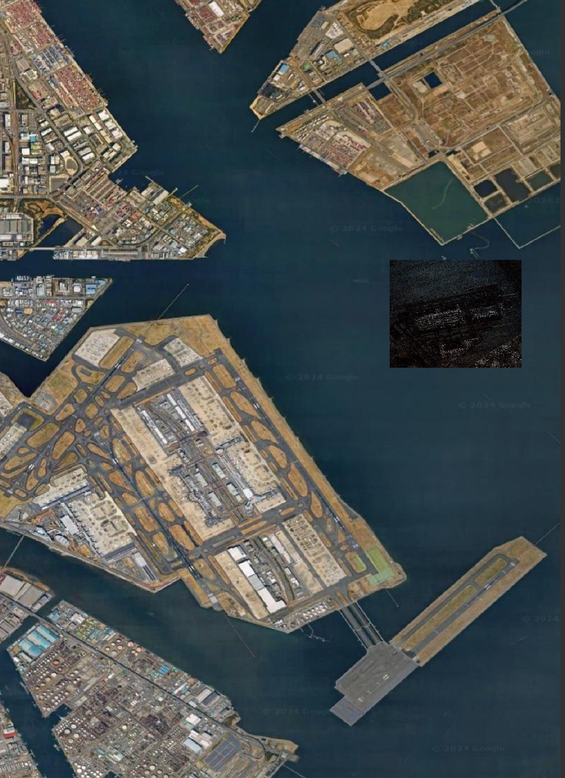
RPC allows for sophisticated and very accurate placement of imagery. Not all tools in GDAL work with RPC out of the box. Issues of misplacement can come up if RPC isn't taken into account when processing imagery through different tooling. Below is an example where Tokyo's Haneda is east of where it should be.
Before working with Umbra's imagery, I'll run it through gdalwarp. This will create a GeoTIFF that will be placed properly without the need for tools to fully understand RPC.
$ gdalwarp \
    -t_srs "EPSG:4326" \
    2024-05-25-15-37-54_UMBRA-06_GEC.tif \
    warped.tif
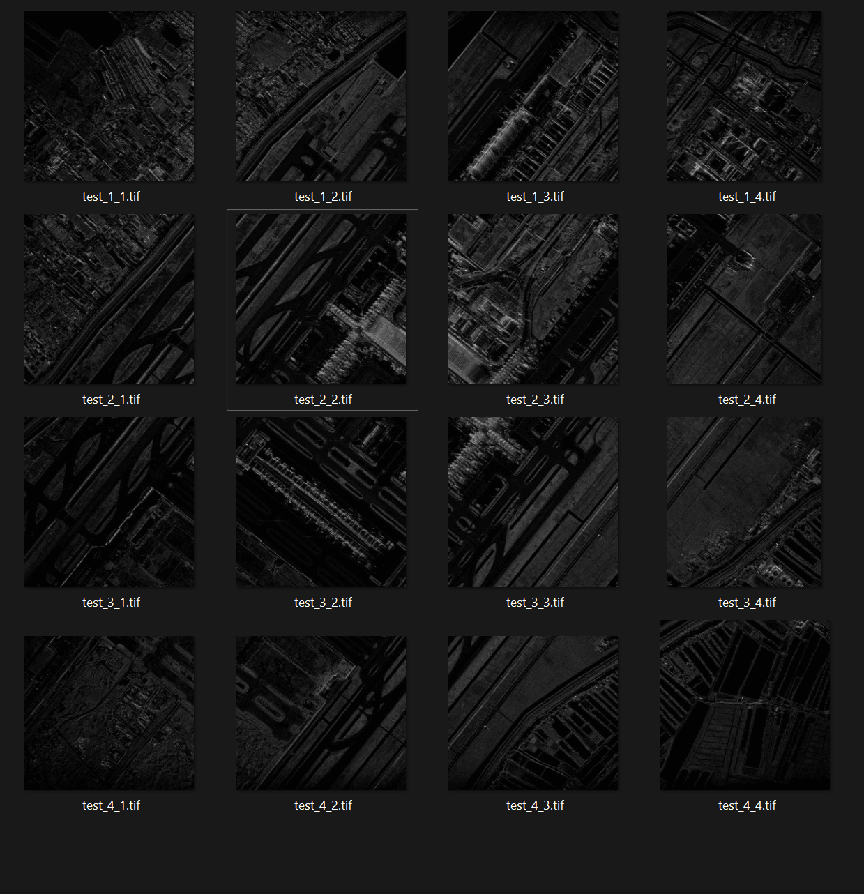
Tiling Imagery
Umbra's images can be 10s of thousands of pixels wide and tall. When I ran this model on the original images, I was seeing fewer items detected than when I broke the image up into smaller tiles. Below I'll break up Umbra's BKK image into 4096x4096-pixel GeoTIFFs.
$ gdal_retile.py \
    -s_srs "EPSG:4326" \
    -ps 4096 4096 \
    -targetDir ./ \
    warped.tif
Below is a screenshot of the tiles.
Inference on Tiles
I'll run DeonDet on each tile and output the results into individual folders. Each folder will include an annotated image as well as a JSON file of the detections.
$ for FILENAME in warped\_*\_*.tif; do
    STEM=`echo "$FILENAME" | grep -o '[0-9]\_[0-9]'`
    echo $STEM
    mkdir -p "out.$STEM"

    python3 \
        ~/SARDet_100K/MSFA/image_demo.py \
        "./$FILENAME" \
        ~/SARDet_100K/MSFA/local_configs/DeonDet/gfl_r50_denodet_sardet.py \
        --weights ~/ckpts/gfl_r50_denodet_sardet/epoch_best.pth \
        --out-dir "out.$STEM"
  done
I wrote a Python script that reads the resulting detections and produces a single GPKG file of them.
$ vi json_to_gpkg.py
import itertools
from   glob             import glob
import json

import geopandas        as gpd
from   osgeo            import gdal
import pandas           as pd
from   shapely.geometry import box
import typer


app = typer.Typer(rich_markup_mode='rich')


def get_coords(mx, my, x_min, x_size, y_min, y_size):
    px = mx * x_size + x_min
    py = my * y_size + y_min

    return px, py


def get_scores(tile='4_3'):
    (x_min,
     x_size,
     _,
     y_min,
     _,
     y_size) = gdal.Open('warped_%s.tif' % tile).GetGeoTransform()

    try:
        recs = json.loads(open('out.%s/preds/warped_%s.json' % (tile, tile)).read())
    except FileNotFoundError: # Inference failed for some reason
        return []

    out = []

    for num, score in enumerate(recs['scores']):
        x1, y1, x2, y2 = recs['bboxes'][num]

        r1 = get_coords(x1, y1, x_min, x_size, y_min, y_size)
        r2 = get_coords(x2, y2, x_min, x_size, y_min, y_size)

        out.append((score, r1[0], r1[1], r2[0], r2[1]))

    return out


@app.command()
def main(out:str):
    tiles = [x.split('.')[0].split('warped_')[-1]
             for x in glob('warped_*_*.tif')]

    res = list(itertools.chain.from_iterable(
                    list(filter(None,
                                [get_scores(tile)
                                 for tile in tiles]))))

    gdf = gpd.GeoDataFrame(
                pd.DataFrame({'score': [x[0] for x in res],
                              'geom':  [box(x[1], x[2], x[3], x[4])
                                       for x in res]}),
                           crs='4326',
                           geometry='geom')
    gdf.to_file(out, driver="GPKG")


if __name__ == "__main__":
    app()
$ python json_to_gpkg.py \
    gfl_r50_denodet_sardet.gpkg
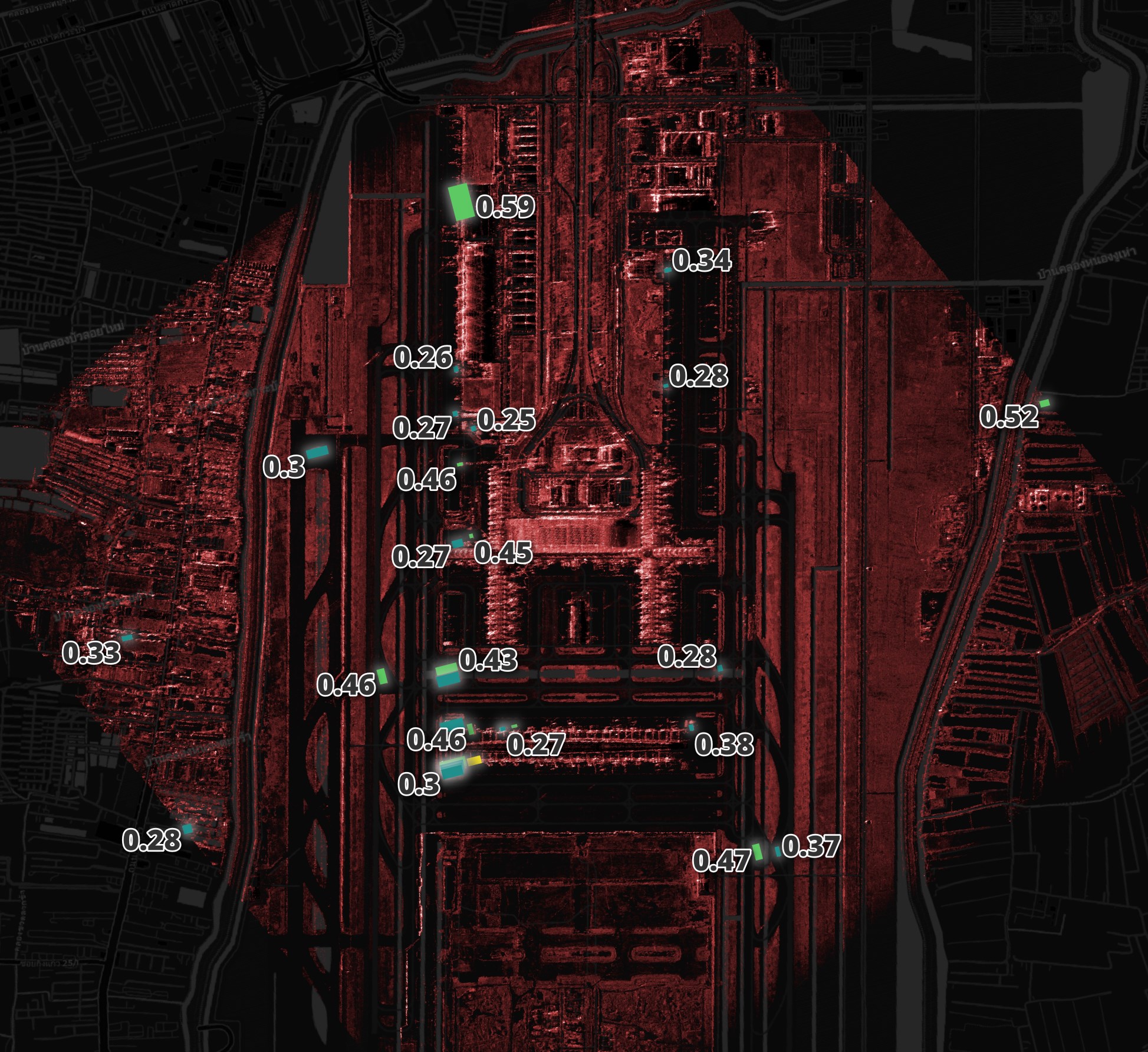
I've disregarded the classes of objects being detected for this exercise. I just wanted to see how many plane parking spots were detected with a decent confidence score.
Most of the 0.4+ scores are in and around the runways, taxi and parking areas.
There aren't many detections around where I suspect there are aircraft. I'll first show an RGB image of the satellite terminal parking area to help give some context.
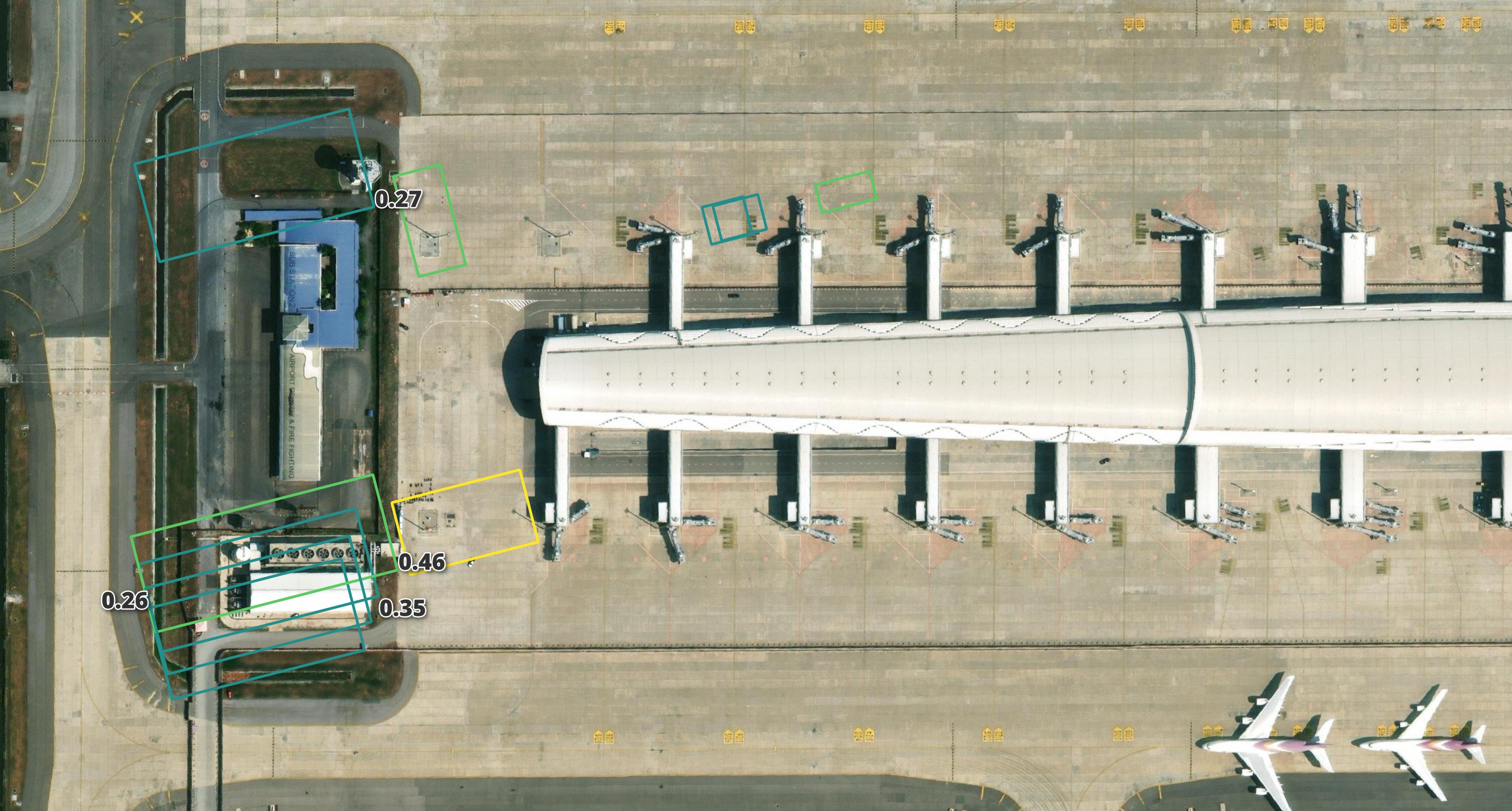
To the right of the image seems to be a lot of aircraft that haven't been detected. It's the same story when I look around the other parking areas in this results set as well.
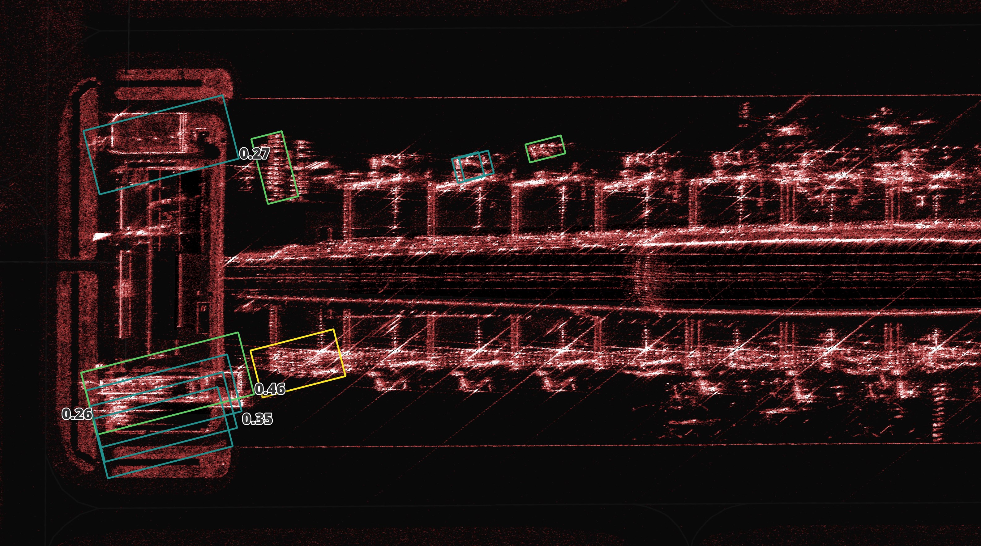
I would accept a lot of permanent infrastructure being falsely detected as an aircraft because I could geofence the results to just the areas aircraft can park or taxi. But in this case, the model is missing the aircraft altogether.
Further Research
As I uncover more insights, I'll update this post with my findings.