Google and Apple are able to innovate in the GIS space due to the vast, global datasets they keep hidden behind their services. Finding global datasets, outside of OpenStreetMap (OSM), is challenging and when the datasets need to be free, the choices are even fewer and further between.
To add to that, OSM won't accept bulk submissions produced by AI, instead wanting each and every change confirmed by a human. Finding volunteers willing to validate 30K building height measurements from LiDAR scans can be far beyond the reach of charity.
But the world of GIS isn't about using a single data provider. GIS is an ecosystem. Using several datasets from a diverse and unaffiliated set of providers is the path to innovation. To add to this, maps are outdated the moment they're published and AI will be key to faster refresh intervals.
The Overture Maps Foundation is a joint development project with the aim of producing global, open map data. The firms partnering with Overture include Amazon, Esri, Meta, Microsoft, Precisely and TomTom. Overture's partner firms have committed to providing funding, engineering and data. When providers are unwilling to publish a proprietary dataset, there are cases where they'll run AI models to produce derivative datasets that will find their way into Overture's published works.
Overture is led by Marc Prioleau, who previously spent four years as the head of business development for Mapping and Location at Meta, five years at Mapbox, including sitting on their Board of Directors and a year at Uber doing business development for their location-based services.
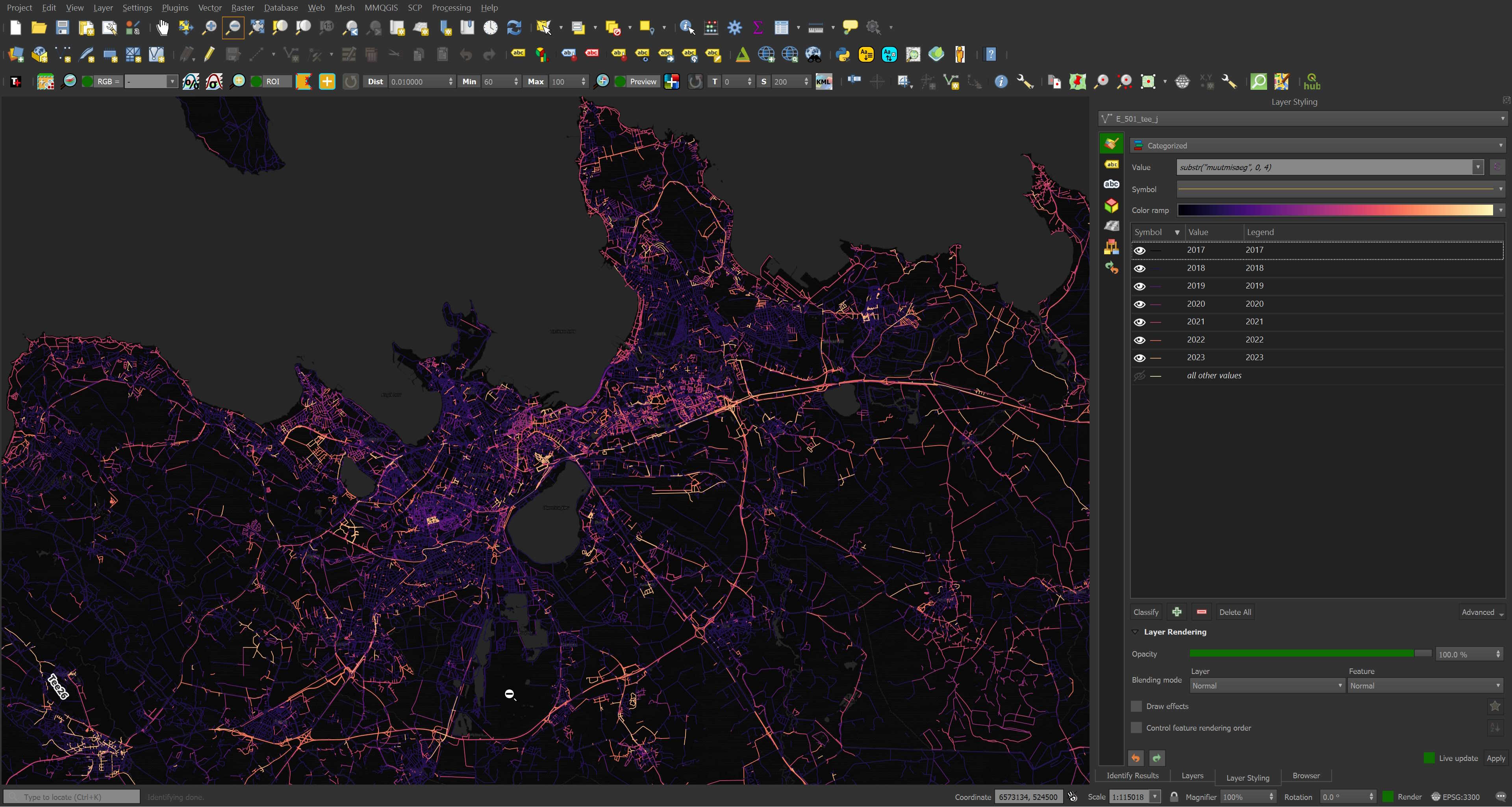
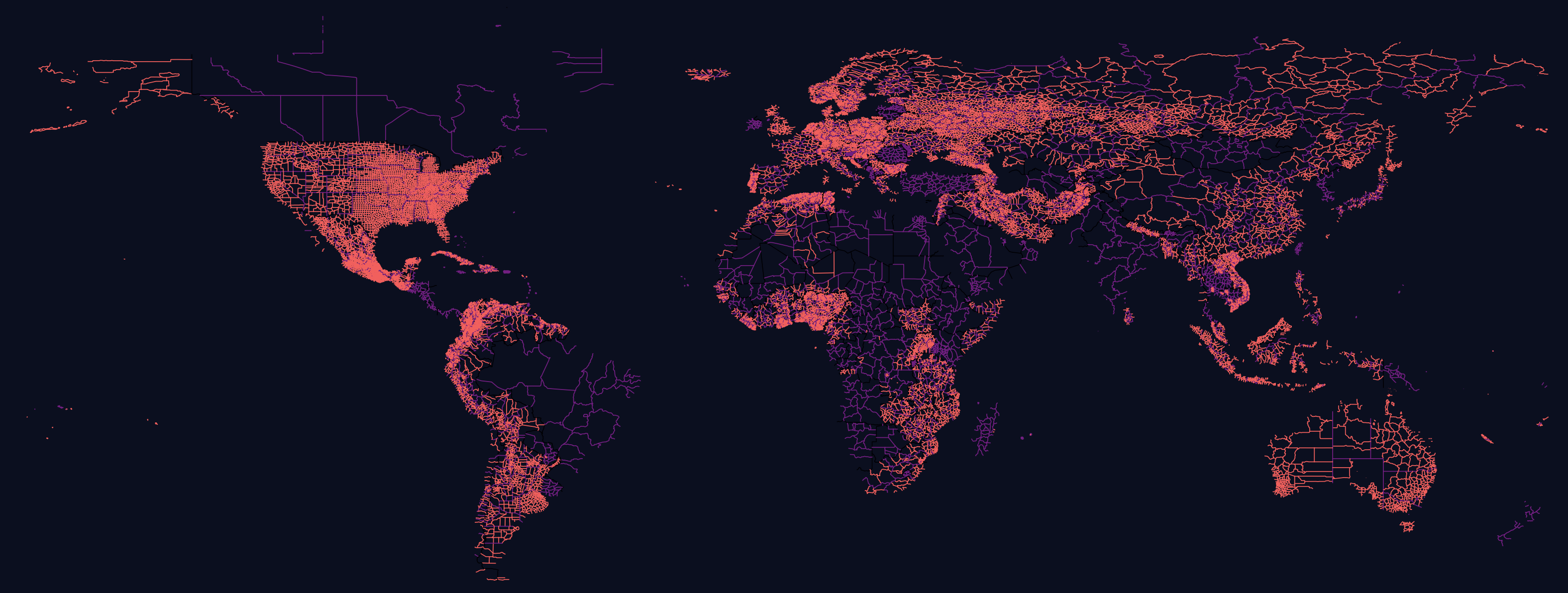
Below is a rendering of Overture's buildings dataset, one of six datasets they released in July of this year. Each building's colour maps to the amount of time since the record's last update. Bright yellow indicates the record has been updated in the past year. The geometry sits on top of CARTO's dark basemap.
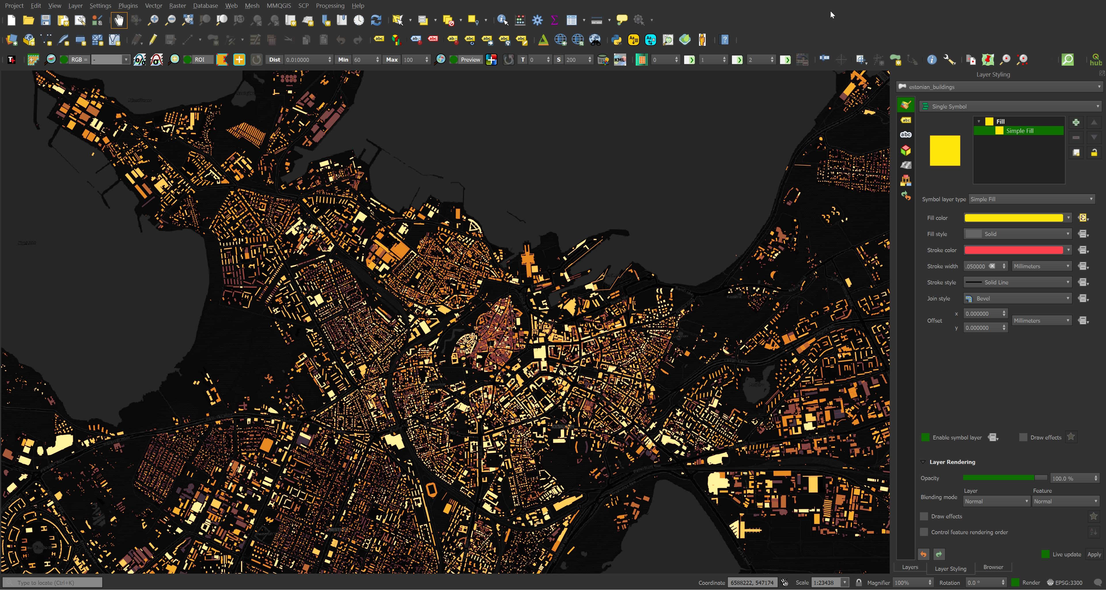
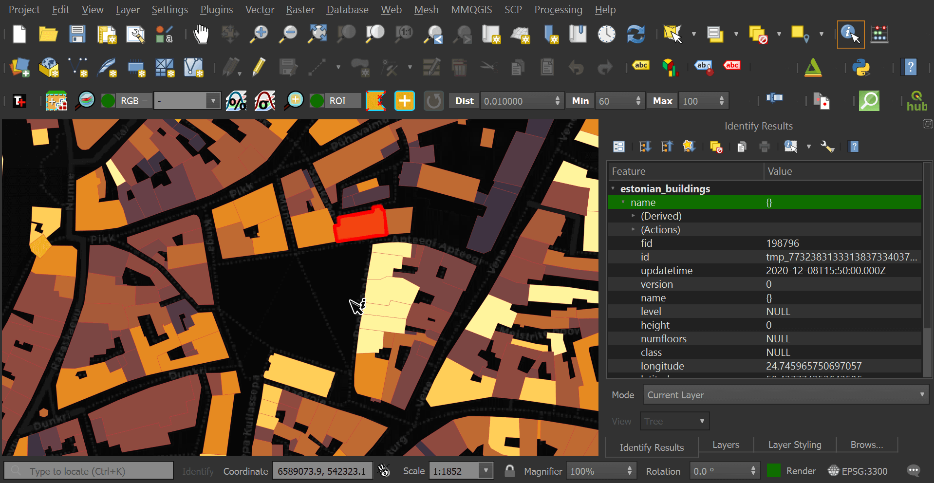
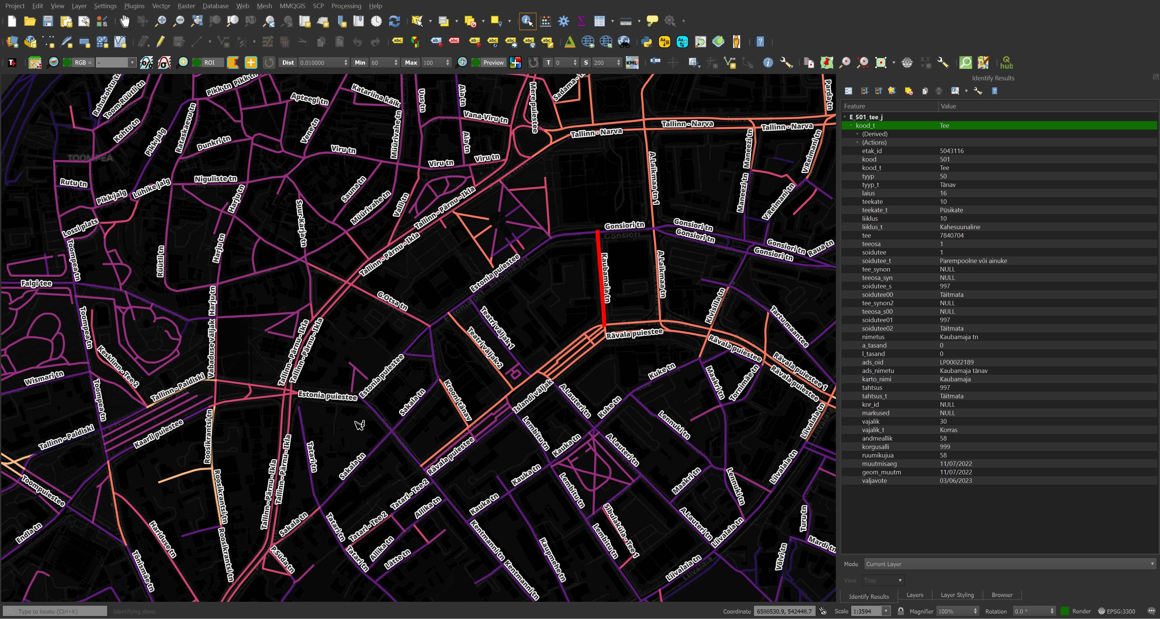
Below is the building that Europe's oldest, continuously operating pharmacy lives within. Even its record was refreshed in December of 2020.
I've spent the last six months working with Overture's three releases they've produced. In this post, I'll go over each of them and dive into the third revision that was published a few weeks ago.
Installing Prerequisites
The following was run on Ubuntu for Windows which is based on Ubuntu 20.04 LTS. The system is powered by an Intel Core i5 4670K running at 3.40 GHz and has 32 GB of RAM. The primary partition is a 2 TB Samsung 870 QVO SSD which will host the DuckDB files produced in this post. The Parquet files in this post will live on an 8 TB mechanical drive.
I'll be using Python and PyArrow to analyse Parquet files as well as GDAL to help out with some transformations in this post.
$ sudo apt update
$ sudo apt install \
    gdal-bin \
    jq \
    python3-pip \
    python3-virtualenv
$ virtualenv ~/.pq
$ source ~/.pq/bin/activate
$ python -m pip install \
    humanize \
    pyarrow
I'll also use DuckDB, along with its JSON, Parquet and Spatial extensions, in this post.
$ cd ~
$ wget -c https://github.com/duckdb/duckdb/releases/download/v0.9.1/duckdb_cli-linux-amd64.zip
$ unzip -j duckdb_cli-linux-amd64.zip
$ chmod +x duckdb
$ ~/duckdb
INSTALL json;
INSTALL parquet;
INSTALL spatial;
I'll set up DuckDB to load all these extensions each time it launches.
$ vi ~/.duckdbrc
.timer on
.width 180
LOAD json;
LOAD parquet;
LOAD spatial;
The maps in this post were rendered with QGIS version 3.32. QGIS is a desktop application that runs on Windows, macOS and Linux.
Overture's April Release
The first release of Overture datasets was in April of this year. It was packaged as an 84 GB, PBF-based OpenStreetMap (OSM) file. The file itself was hosted on an AWS S3 HTTPS link rather than a CDN. The geometry within it was projected to EPSG:3857 and if you wanted to import it into BigQuery you had to re-projecting it to EPSG:4326.
I've yet to find a tool that reads PBF-based OSM files that can take advantage of modern hardware. I ended up waiting almost six days for osm2pgsql to import the file into PostgreSQL.
$ createdb overture
$ echo "CREATE EXTENSION postgis;" \
    | psql overture
$ osm2pgsql -d overture \
            --slim \
            --drop \
            planet-2023-04-02-alpha.osm.pbf
The resulting tables were between 12 and 205 GB each in PostgreSQL's internal storage format.
  Size | Table
-------|------
205 GB | planet_osm_polygon
 92 GB | planet_osm_line
 14 GB | planet_osm_point
 12 GB | planet_osm_roads
Overture's July Release
In July, Overture released a second iteration of their datasets, this time in Parquet format and totalling a little over 200 GB.
This release was made available via an AWS S3 bucket. Downloading the data via aws s3 sync wasn't able to saturate my half-gigabit connection but I was able to pull the data down at ~13-15 MB/s which is around 4x faster than pulling from AWS S3 via HTTPS with wget or curl.
Below is a breakdown of the file sizes of each of the datasets.
  Size | Table
-------|------
110 GB | Buildings
 63 GB | Transport Segments
 20 GB | Transport Connectors
  8 GB | Places
0.5 GB | Local Administrations
0.1 GB | Administrative Boundaries
The bulk of the buildings data came from OpenStreetMap, Microsoft's ML Buildings, Esri's Community Maps and USGS' LiDAR datasets. TomTom provided the administrative boundaries. Transport connectors and segments are from OpenStreetMap. Meta and Microsoft produced the Places dataset. The Locality datasets are from Esri and TomTom.
Using Parquet over S3 means it's possible to both query local files as well as files residing on S3 with DuckDB. Parquet stores data more efficiently as columns rather than rows with each column containing summary statistics every few thousand values.
Storing data this way makes it easier for compressors, like GZIP and ZStandard, to shrink the size of the dataset. ZStandard does a good job of taking advantage of modern hardware and should decompress ~3x faster than GZIP when reading the data back.
This means a minimal amount of I/O and compute will be needed to ask certain questions that don't rely on reading a column's data outright and if data did need to be read in full, only the column(s) in question would be read, not the full record.
Each of the six datasets is made up of ~30 to 120 Parquet files. Records aren't sorted by geography and records covering a ~6 KM radius can span across every file in the dataset. Below I'll count the number of building records in the centre of in Tallinn across each Parquet file.
$ cd ~/overture_2023_07/theme=buildings/type=building
$ ~/duckdb
SELECT filename,
       COUNT(*)
FROM READ_PARQUET('202307*', filename=true)
WHERE ST_DISTANCE(ST_POINT(24.7389, 59.4509),
                  ST_CENTROID(ST_GEOMFROMWKB(geometry))) < 0.129
GROUP BY 1
ORDER BY 2 DESC;
┌──────────────────────────────────────────────────────────────────┬──────────────┐
│                             filename                             │ count_star() │
│                             varchar                              │    int64     │
├──────────────────────────────────────────────────────────────────┼──────────────┤
│ 20230725_211555_00082_tpd52_72d91b5f-c33d-40e7-9df3-703b268bc3ed │          585 │
│ 20230725_211555_00082_tpd52_1d174ef1-dd7c-45f5-9431-81b4dd8411a3 │          575 │
│ 20230725_211555_00082_tpd52_7d00c15a-97f9-4497-8b72-eeb6aa6f5d20 │          573 │
│ 20230725_211555_00082_tpd52_c95a8578-9ecb-4eae-a53e-c154fc138009 │          573 │
│ 20230725_211555_00082_tpd52_1dbc92a9-9bb9-404c-99a5-f14ff648eca1 │          572 │
│ 20230725_211555_00082_tpd52_a69debf5-a538-407a-93bd-cb7293090185 │          572 │
│ 20230725_211555_00082_tpd52_c39b517a-5b57-4e3b-bc4b-528099fd0997 │          571 │
│ 20230725_211555_00082_tpd52_c843adcb-8d10-48e4-b476-212d71b61af1 │          568 │
│ 20230725_211555_00082_tpd52_d1c2dcd1-89ff-4a89-8134-1075b08cbd78 │          564 │
│ 20230725_211555_00082_tpd52_b95d355a-b594-437f-b1b2-500162cbc636 │          562 │
│ 20230725_211555_00082_tpd52_ffe10440-d4ef-474f-aff8-99bd14a9517d │          562 │
│ 20230725_211555_00082_tpd52_8b590512-3e53-47f3-9854-b99f246b418b │          560 │
│ 20230725_211555_00082_tpd52_498b7931-9b43-4eb1-9da2-d995d3032a60 │          559 │
│ 20230725_211555_00082_tpd52_58f3983e-7655-4a46-8e0c-5527d4d9e870 │          559 │
│ 20230725_211555_00082_tpd52_9a267136-5e70-48b2-993d-5139be3b695b │          558 │
│ 20230725_211555_00082_tpd52_ee792775-d04b-43b1-b712-9de7a29e7ad1 │          558 │
│ 20230725_211555_00082_tpd52_99c95261-d5ad-4fa5-ab5e-9a93861c29de │          558 │
│ 20230725_211555_00082_tpd52_142f876e-aaaf-4c15-a27f-9ee8d5d6831e │          558 │
│ 20230725_211555_00082_tpd52_c0841271-76c7-4d94-aeea-2d63fe9e3480 │          555 │
│ 20230725_211555_00082_tpd52_4dc6891c-f25b-47f5-83f8-64cb6c31d476 │          554 │
│                                ·                                 │           ·  │
│                                ·                                 │           ·  │
│                                ·                                 │           ·  │
│ 20230725_211555_00082_tpd52_ce1defc0-17b2-4c09-88c0-97a48f541ade │          167 │
│ 20230725_211555_00082_tpd52_6a8dd31f-0a60-4d32-830e-0b66fbde3d64 │          148 │
│ 20230725_211555_00082_tpd52_2161a94f-857c-4cbe-86ab-15f4be7c7d35 │          140 │
│ 20230725_211555_00082_tpd52_429747ee-1d9e-409d-a6d3-ec293fc4d68b │          136 │
│ 20230725_211555_00082_tpd52_2a8621dd-ea8d-46c2-b3d3-2caebab533a2 │          134 │
│ 20230725_211555_00082_tpd52_74494bd4-86ff-47e8-bda5-8649ef1a832e │          131 │
│ 20230725_211555_00082_tpd52_5e02b9a3-f430-4a78-b886-41844d16cca0 │          129 │
│ 20230725_211555_00082_tpd52_cb60d49e-a2df-4014-83c7-3668cc3d6a3e │          126 │
│ 20230725_211555_00082_tpd52_1d65a4ac-16e8-49a1-a3a0-a1e2aca72c74 │          124 │
│ 20230725_211555_00082_tpd52_732a7836-7733-43b0-98c7-7fde503ad887 │          123 │
│ 20230725_211555_00082_tpd52_ad45683d-c24c-4fef-8569-cc1d48318522 │          119 │
│ 20230725_211555_00082_tpd52_ae6b950d-6160-4341-9487-751e7e0f8f79 │          109 │
│ 20230725_211555_00082_tpd52_5ef05d8c-f7cd-4e4c-a493-fc1fe7458585 │          106 │
│ 20230725_211555_00082_tpd52_9780f848-4fd2-43f8-82e6-58b09a6f6862 │          100 │
│ 20230725_211555_00082_tpd52_b3636f25-196e-4ff1-bbe6-97ed5591c5e5 │           96 │
│ 20230725_211555_00082_tpd52_0eb57855-f854-47b0-a38b-c248804e8222 │           96 │
│ 20230725_211555_00082_tpd52_d6b3ff3b-7c33-4579-a4d7-ac72ecb042ab │           86 │
│ 20230725_211555_00082_tpd52_e540e2da-f80b-483c-9f2b-8cd43fa52271 │           78 │
│ 20230725_211555_00082_tpd52_59160cd7-f19b-4806-83b2-200b5d14df17 │           73 │
│ 20230725_211555_00082_tpd52_5f8e2d88-86c3-4106-94f6-cd857c58c4ba │           53 │
├──────────────────────────────────────────────────────────────────┴──────────────┤
│ 120 rows (40 shown)                                                   2 columns │
└─────────────────────────────────────────────────────────────────────────────────┘
Spatial Lookups
If you're working with a field within a Parquet file or group of files then certain queries can be answered quickly from column statistics alone. The following could potentially only need to read KBs of data out of the 110 GB Buildings dataset.
SELECT MAX(height)
FROM   READ_PARQUET('202307*');
Unfortunately, this doesn't seem to extend itself to the bounding box's structure. The following took ages to complete on my system.
SELECT   filename,
         COUNT(*)
FROM     READ_PARQUET('202307*', filename=true)
WHERE    26 > bbox.minx AND bbox.minx > 24
AND      60 > bbox.miny AND bbox.miny > 58
GROUP BY 1
ORDER BY 2 DESC;
Using the Spatial Extension's functions on the bounding box field didn't help speed anything up either. The lookup for Tallinn buildings using the ST_DISTANCE function took over 35 minutes to complete.
It would be great if there were centroid_x and centroid_y fields in each of these datasets that could be used as predicates. This could go a long way to extracting out records of interest a lot faster.
Large Row Groups
One thing I would have liked to see in the July release is smaller row groups. These allow skipping over data that might not be of interest and can save a lot of I/O and/or bandwidth.
Below is one of the buildings files and with 8,020,380 records and only ten row groups. I'm used to seeing row groups max out at 10-15K values so having groups span 891,399 values is really strange. Given the underlying data in any one column isn't likely to be sorted, this can make finding row groups that can be skipped over much more difficult.
$ python3
from collections import Counter
from operator    import itemgetter
from pprint      import pprint

import pyarrow.parquet as pq


pf = pq.ParquetFile('20230725_211555_00082_tpd52_00e93efa-24f4-4014-b65a-38c7d2854ab4')

print(pf.metadata)
<pyarrow._parquet.FileMetaData object at 0x7f9204339c70>
  created_by: parquet-mr version 1.12.2-amzn-athena-1 (build 6c6353027ef5d7782e8657ea59b290452cdfdaee)
  num_columns: 17
  num_rows: 8020380
  num_row_groups: 10
  format_version: 1.0
  serialized_size: 36789
print(Counter(pf.metadata.row_group(rg).num_rows
              for rg in range(0, pf.metadata.num_row_groups)))
Counter({891399: 8, 888014: 1, 1174: 1})
Only around 25% of the row groups achieved a compression ratio of 3:1 or better. I suspect using a different sort key could achieve a better ratio.
ratios = []

for rg in range(0, pf.metadata.num_row_groups):
    for col in range(0, pf.metadata.num_columns):
        x = pf.metadata.row_group(rg).column(col)
        ratio = x.total_uncompressed_size / x.total_compressed_size
        ratios.append(float('%.1f' % ratio))

pprint(sorted(Counter(ratios).items(),
              key=itemgetter(0)))
[(0.8, 20),
 (1.0, 21),
 (1.1, 21),
 (1.2, 3),
 (1.3, 1),
 (1.4, 10),
 (1.5, 18),
 (1.7, 3),
 (1.8, 24),
 (2.2, 9),
 (2.3, 1),
 (3.2, 1),
 (3.3, 1),
 (3.5, 9),
 (4.8, 9),
 (5.0, 9),
 (6.4, 1),
 (14.1, 2),
 (14.2, 6),
 (14.3, 1)]
I tried sorting by location in one of the Parquet files as it'll provide better patterns in the lengthy geometry field for ZStandard to spot. The following reduced the Parquet file's size by 7% while providing a smaller row group size and casting the update time from a string to a timestamp. The file size would be just about identical if I had left the centroid fields in.
CREATE OR REPLACE TABLE test AS
    SELECT * EXCLUDE (updatetime),
           updatetime::TIMESTAMP updatetime,
           ST_X(ST_CENTROID(ST_GEOMFROMWKB(geometry))) centroid_x,
           ST_Y(ST_CENTROID(ST_GEOMFROMWKB(geometry))) centroid_y
    FROM READ_PARQUET('20230725_211555_00082_tpd52_5f8e2d88-86c3-4106-94f6-cd857c58c4ba');

COPY (SELECT * EXCLUDE (centroid_x,
                        centroid_y)
      FROM test
      ORDER BY centroid_x,
               centroid_y)
TO 'test.pq' (FORMAT 'PARQUET',
              CODEC  'ZSTD',
              ROW_GROUP_SIZE 15000);
Overture's October Release
In October, a third, 327 GB release was published by Overture. This time, they created a unified schema across all the datasets.
$ mkdir -p ~/overture_2023_10
$ cd ~/overture_2023_10
$ aws s3 sync \
    --no-sign-request \
    s3://overturemaps-us-west-2/release/2023-10-19-alpha.0/ \
    ./
Below is a breakdown of the file sizes of each of the datasets.
  Size | Table
-------|------
176 GB | Buildings
 62 GB | Transport Segments
 25 GB | Land
 20 GB | Water
 20 GB | Transport Connectors
 16 GB | Land-use
  7 GB | Places
  2 GB | Local Administrations
0.4 GB | Administrative Boundaries
I'll load a single record into a new DuckDB table so we can examine the schema. The CREATE TABLE schema was formatted for better readability.
$ ~/duckdb
CREATE OR REPLACE TABLE overture AS
    SELECT *
    FROM READ_PARQUET('theme=buildings/type=building/part-02387-*.c000.zstd.parquet')
    LIMIT 1;

.schema --indent
CREATE TABLE overture (
  categories
    STRUCT(main      VARCHAR,
           alternate VARCHAR[]),
  "level"              INTEGER,
  socials              VARCHAR[],
  subType              VARCHAR,
  numFloors            INTEGER,
  entityId             VARCHAR,
  "class"              VARCHAR,
  sourceTags           MAP(VARCHAR, VARCHAR),
  localityType         VARCHAR,
  emails               VARCHAR[],
  drivingSide          VARCHAR,
  adminLevel           INTEGER,
  road                 VARCHAR,
  isoCountryCodeAlpha2 VARCHAR,
  isoSubCountryCode    VARCHAR,
  updateTime           VARCHAR,
  wikidata             VARCHAR,
  confidence           DOUBLE,
  defaultLanguage      VARCHAR,
  brand
    STRUCT("names"
        STRUCT(common    STRUCT("value" VARCHAR, "language" VARCHAR)[],
               official  STRUCT("value" VARCHAR, "language" VARCHAR)[],
               alternate STRUCT("value" VARCHAR, "language" VARCHAR)[],
               short     STRUCT("value" VARCHAR, "language" VARCHAR)[]),
               wikidata  VARCHAR),
  addresses
    STRUCT(freeform VARCHAR,
           locality VARCHAR,
           postCode VARCHAR,
           region   VARCHAR,
           country  VARCHAR)[],
  "names"
    STRUCT(common    STRUCT("value" VARCHAR, "language" VARCHAR)[],
           official  STRUCT("value" VARCHAR, "language" VARCHAR)[],
           alternate STRUCT("value" VARCHAR, "language" VARCHAR)[],
           short     STRUCT("value" VARCHAR, "language" VARCHAR)[]),
  isIntermittent       BOOLEAN,
  connectors           VARCHAR[],
  surface              VARCHAR,
  "version"            INTEGER,
  phones               VARCHAR[],
  id                   VARCHAR,
  geometry             BLOB,
  context              VARCHAR,
  height               DOUBLE,
  maritime             BOOLEAN,
  sources
    STRUCT(property   VARCHAR,
           dataset    VARCHAR,
           recordId   VARCHAR,
           confidence DOUBLE)[],
  websites             VARCHAR[],
  isSalt               BOOLEAN,
  bbox
    STRUCT(minx DOUBLE,
           maxx DOUBLE,
           miny DOUBLE,
           maxy DOUBLE)
);;
Below are all of the non-NULL fields in the first building record. The output was formatted for readability.
.mode line

SELECT updateTime,
       names,
       id,
       ST_GEOMFROMWKB(geometry) geom,
       sources,
       bbox
FROM overture;
updateTime = 2022-09-28T23:07:45.000Z
     names = {'common': [],
              'official': [],
              'alternate': [],
              'short': []}
        id = w1098690595@1
      geom = POLYGON ((23.2530373 41.2662782,
                       23.2530422 41.2661573,
                       23.2531882 41.2661606,
                       23.2531833 41.2662815,
                       23.2530373 41.2662782))
   sources = [{'property': ,
               'dataset': OpenStreetMap,
               'recordId': w1098690595@1,
               'confidence': NULL}]
      bbox = {'minx': 23.2530373,
              'maxx': 23.2531882,
              'miny': 41.2661573,
              'maxy': 41.2662815}
The following is the number of compressed and uncompressed bytes for each column. This list has been truncated to the top 15 columns by number of compressed bytes.
from glob        import glob

from humanize import naturalsize


columns = {}

for filename in glob('theme=*/type=*/part-*.zstd.parquet'):
    pf = pq.ParquetFile(filename)

    for rg in range(0, pf.metadata.num_row_groups):
        for col in range(0, pf.metadata.num_columns):
            col_data = pf.metadata.row_group(rg).column(col)
            key = col_data.path_in_schema

            if key not in columns.keys():
                columns[key] = {'compressed': 0,
                                'uncompressed': 0}

            columns[key]['compressed'] = \
                columns[key]['compressed'] + \
                col_data.total_compressed_size
            columns[key]['uncompressed'] = \
                columns[key]['uncompressed'] + \
                col_data.total_uncompressed_size

for rec in sorted([(x[0],
                    x[1]['compressed'],
                    x[1]['uncompressed'])
                   for x in columns.items()],
                  key=itemgetter(1),
                  reverse=True)[:15]:
    print('%10s | %10s | %s' % (naturalsize(rec[1]),
                                naturalsize(rec[2]),
                                rec[0]))
compressed | uncompressed | field name
-----------|--------------|-----------
  214.3 GB |     286.4 GB | geometry
   32.7 GB |      74.1 GB | id
   16.8 GB |      17.9 GB | bbox.maxx
   16.8 GB |      17.9 GB | bbox.minx
   16.4 GB |      17.9 GB | bbox.miny
   16.4 GB |      17.9 GB | bbox.maxy
   12.7 GB |      30.0 GB | sources.list.element.recordId
   11.9 GB |      34.2 GB | connectors.list.element
    4.5 GB |      36.3 GB | updateTime
    2.6 GB |      18.6 GB | road
    1.2 GB |       2.2 GB | names.common.list.element.value
  733.1 MB |       1.4 GB | addresses.list.element.freeform
  517.0 MB |       1.4 GB | websites.list.element
  486.9 MB |       2.3 GB | socials.list.element
  321.2 MB |     765.3 MB | phones.list.element
Even Larger Row Groups
I had a quick look at the row group counts in building Parquet files and saw that there are a maximum of two row groups in any one Parquet file.
$ python3
from collections import Counter
from glob        import glob
from operator    import itemgetter
from pprint      import pprint

import pyarrow.parquet as pq


print(set([pq.ParquetFile(x).metadata.num_row_groups
           for x in glob('part*parquet')]))
{1, 2}
When inspecting an individual file I can see the parquet writer's signature has changed since the July release.
pf = pq.ParquetFile('part-02355-87dd7d19-acc8-4d4f-a5ba-20b407a79638.c000.zstd.parquet')

print(pf.metadata)
<pyarrow._parquet.FileMetaData object at 0x7f4a280b1bd0>
  created_by: parquet-mr compatible Photon version 0.2
  num_columns: 63
  num_rows: 1149535
  num_row_groups: 2
  format_version: 1.0
  serialized_size: 17502
This Parquet file has 962,560 records in one row group and 186,975 in the other.
print(Counter(pf.metadata.row_group(rg).num_rows
              for rg in range(0, pf.metadata.num_row_groups)))
Counter({962560: 1, 186975: 1})
With row groups this large, it's unlikely any query will be able to skip over any group when trying to track down records of interest.
Extracting Tallinn's Data
Overture is working on a record identification system called Global Entity Reference System (GERS). The identifiers will look like the following.
8844c0b1a7fffff-17fff78c078ff50b
The first 15 hexadecimal characters reflect the record's H3 spatial index location. GERS should be useable as a fast predicate when scanning Overture's Parquet files for specific geographies. But as of this writing, it hasn't fully rolled out so for now I'm left with extracting points out of either the bounding box or calculating each geometry record's centroid.
I'll extract every record within ~6 KM of Tallinn's Old Town using DuckDB. There is a substantial amount of random I/O needed to produce the DuckDB file so I've placed it on an SSD.
$ ~/duckdb ~/Downloads/tallinn.duckdb
CREATE OR REPLACE TABLE tallinn AS
    SELECT * EXCLUDE (geometry),
           ST_GEOMFROMWKB(geometry) geom
    FROM READ_PARQUET('theme=*/type=*/part*.zstd.parquet',
                      filename=true,
                      hive_partitioning=1)
    WHERE ST_DISTANCE(
              ST_POINT(24.746, 59.4377),
              ST_CENTROID(ST_GEOMFROMWKB(geometry))) < 0.129;
The above finished in 3 hours and 20 minutes and produced a 47 MB DuckDB file with 214,581 records. Here is a breakdown of the record types.
SELECT COUNT(*),
       "type"
FROM tallinn
GROUP BY 2
ORDER BY 1 DESC;
┌──────────────┬────────────────────────┐
│ count_star() │          type          │
│    int64     │        varchar         │
├──────────────┼────────────────────────┤
│        66131 │ connector              │
│        55008 │ building               │
│        39665 │ segment                │
│        22927 │ land                   │
│        17614 │ place                  │
│        12043 │ landuse                │
│         1083 │ water                  │
│          107 │ locality               │
│            3 │ administrativeBoundary │
└──────────────┴────────────────────────┘
I'll dump the table into a GeoPackage file. There are multiple date formats being used so I'll extract the year from them for the time being.
COPY (
    SELECT * EXCLUDE (updateTime,
                      addresses,
                      bbox,
                      brand,
                      categories,
                      connectors,
                      emails,
                      "names",
                      phones,
                      socials,
                      sources,
                      sourceTags,
                      websites),
           REGEXP_EXTRACT(updateTime,
                          '([0-9]{4})')::int updated_year,
           JSON(addresses)  addresses,
           JSON(brand)      brand,
           JSON(categories) categories,
           JSON(connectors) connectors,
           JSON(emails)     emails,
           JSON("names")    "names",
           JSON(phones)     phones,
           JSON(socials)    socials,
           JSON(sources)    sources,
           JSON(sourceTags) sourceTags,
           JSON(websites)   websites
      FROM tallinn
) TO 'tallinn.gpkg'
WITH (FORMAT GDAL,
      DRIVER 'GPKG');
The above produced a 121 MB GeoPackage file in 43 minutes and 12 seconds. I'm not completely sure why it took that long so I'll be producing CSV extracts for any iterations below. GeoPackage files are very performant with QGIS so it's a shame they can't be produced in a shorter time frame.
Below is a breakdown of the record counts for each geometry type for each dataset.
SELECT REPLACE(ST_GeometryType(geom),
               'MULTI',
               '') geom_type,
       "type",
       COUNT(*)
FROM tallinn
GROUP BY 1, 2
ORDER BY 2, 1 DESC;
┌────────────┬────────────────────────┬──────────────┐
│ geom_type  │          type          │ count_star() │
│  varchar   │        varchar         │    int64     │
├────────────┼────────────────────────┼──────────────┤
│ LINESTRING │ administrativeBoundary │            3 │
│ POLYGON    │ building               │        55008 │
│ POINT      │ connector              │        66131 │
│ POLYGON    │ land                   │        10315 │
│ POINT      │ land                   │        12039 │
│ LINESTRING │ land                   │          573 │
│ POLYGON    │ landuse                │        11677 │
│ POINT      │ landuse                │            1 │
│ LINESTRING │ landuse                │          365 │
│ POLYGON    │ locality               │           17 │
│ POINT      │ locality               │           90 │
│ POINT      │ place                  │        17614 │
│ LINESTRING │ segment                │        39665 │
│ POLYGON    │ water                  │          260 │
│ POINT      │ water                  │            7 │
│ LINESTRING │ water                  │          816 │
├────────────┴────────────────────────┴──────────────┤
│ 16 rows                                  3 columns │
└────────────────────────────────────────────────────┘
Below are the data providers for each of the datasets. OpenStreetMap is listed in both singular and plural for some reason.
SELECT DISTINCT UNNEST(sources).dataset,
                "type"
FROM tallinn
ORDER BY 2;
┌───────────────────────────┬────────────────────────┐
│ (unnest(sources)).dataset │          type          │
│          varchar          │        varchar         │
├───────────────────────────┼────────────────────────┤
│ OpenStreetMaps            │ administrativeBoundary │
│ OpenStreetMap             │ building               │
│ OpenStreetMap             │ connector              │
│ OpenStreetMap             │ land                   │
│ OpenStreetMap             │ landuse                │
│ OpenStreetMaps            │ locality               │
│ Esri Community Maps       │ locality               │
│ msft                      │ place                  │
│ meta                      │ place                  │
│ OpenStreetMap             │ segment                │
│ OpenStreetMap             │ water                  │
├───────────────────────────┴────────────────────────┤
│ 11 rows                                  2 columns │
└────────────────────────────────────────────────────┘
Overture's Segments Dataset
The segments / roads data is made up of line strings provided by OSM. They all have the update timestamp of 2023-09-30 21:43:42 UTC. Below I'll prepare a CSV of each road's geometry, name and speed limit as doing this in QGIS alone is beyond the scope of my skill set at the moment.
COPY (
    SELECT geom wkt,
           IFNULL(JSON_EXTRACT(JSON(road),
                               '/restrictions/speedLimits/maxSpeed/0'), 999) max_speed,
           IFNULL(REPLACE(JSON_EXTRACT(JSON(road),
                                       '/roadNames/common/0/value'), '"', ''), 'UNKNOWN') road_name
    FROM tallinn
    WHERE "type" = 'segment'
) TO 'roads.csv'
  WITH (HEADER);
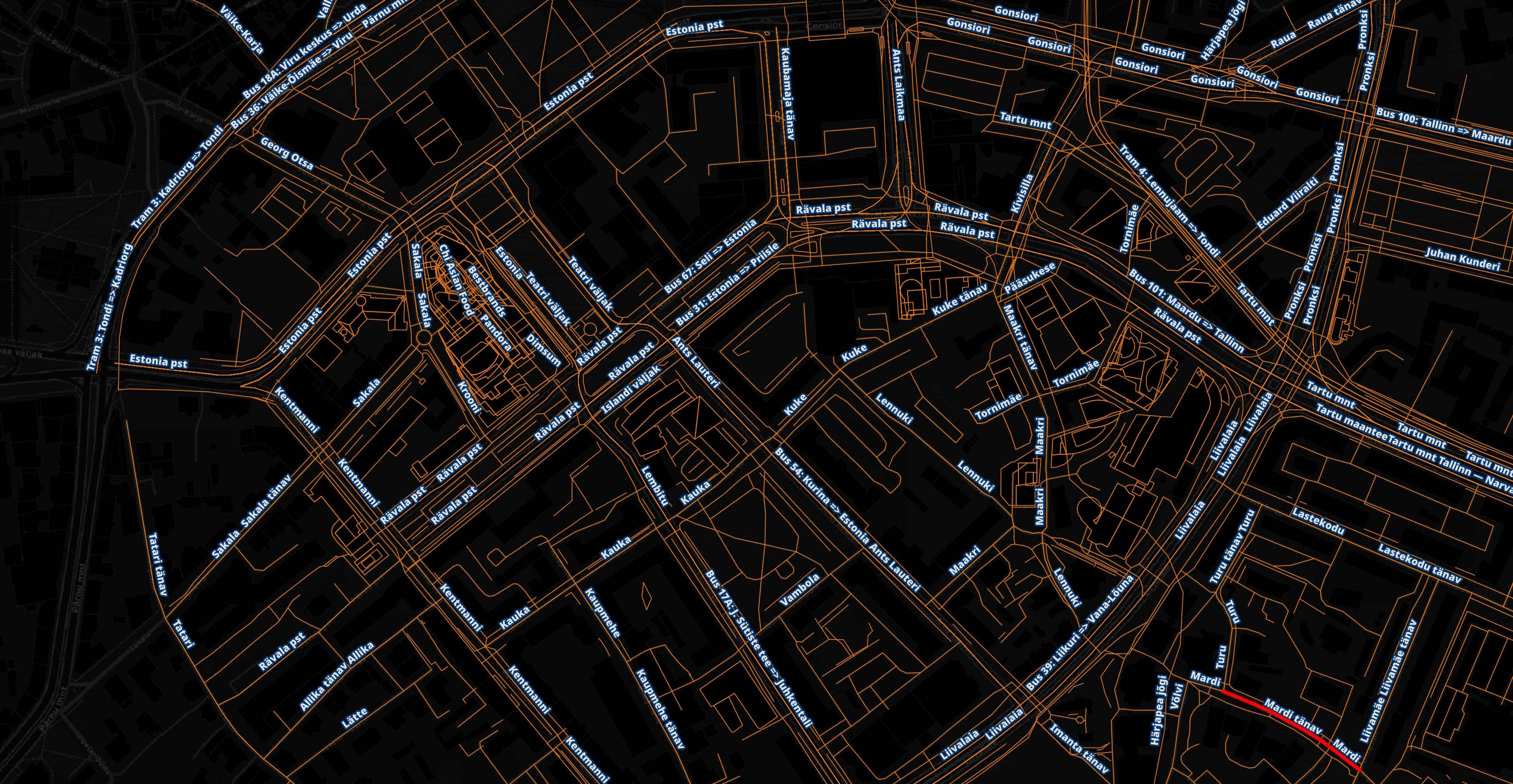
I've coloured the roads in central Tallinn based on their speed limit listed in the dataset and if it's missing they're coloured dark purple. I've also added the street names or set the street's label to 'UNKNOWN'.
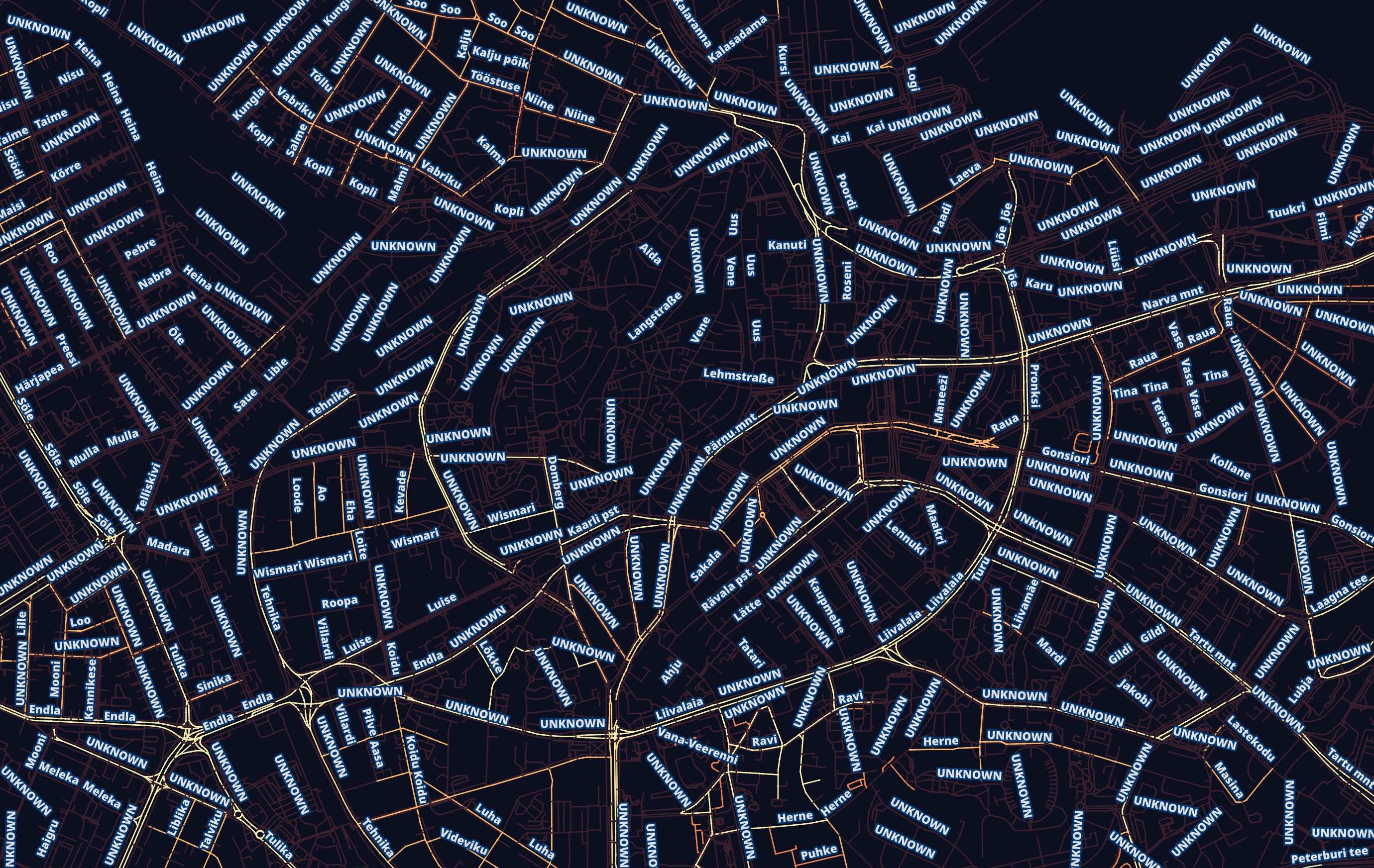
It's great to have geometry for most of the world's roads in one dataset but the metadata gaps for Estonia specifically are too great for any use case I can think of. The Estonian Land Board has Shapefiles documenting every road in the country with in-depth metadata available for free and is a much more complete and comprehensive dataset.
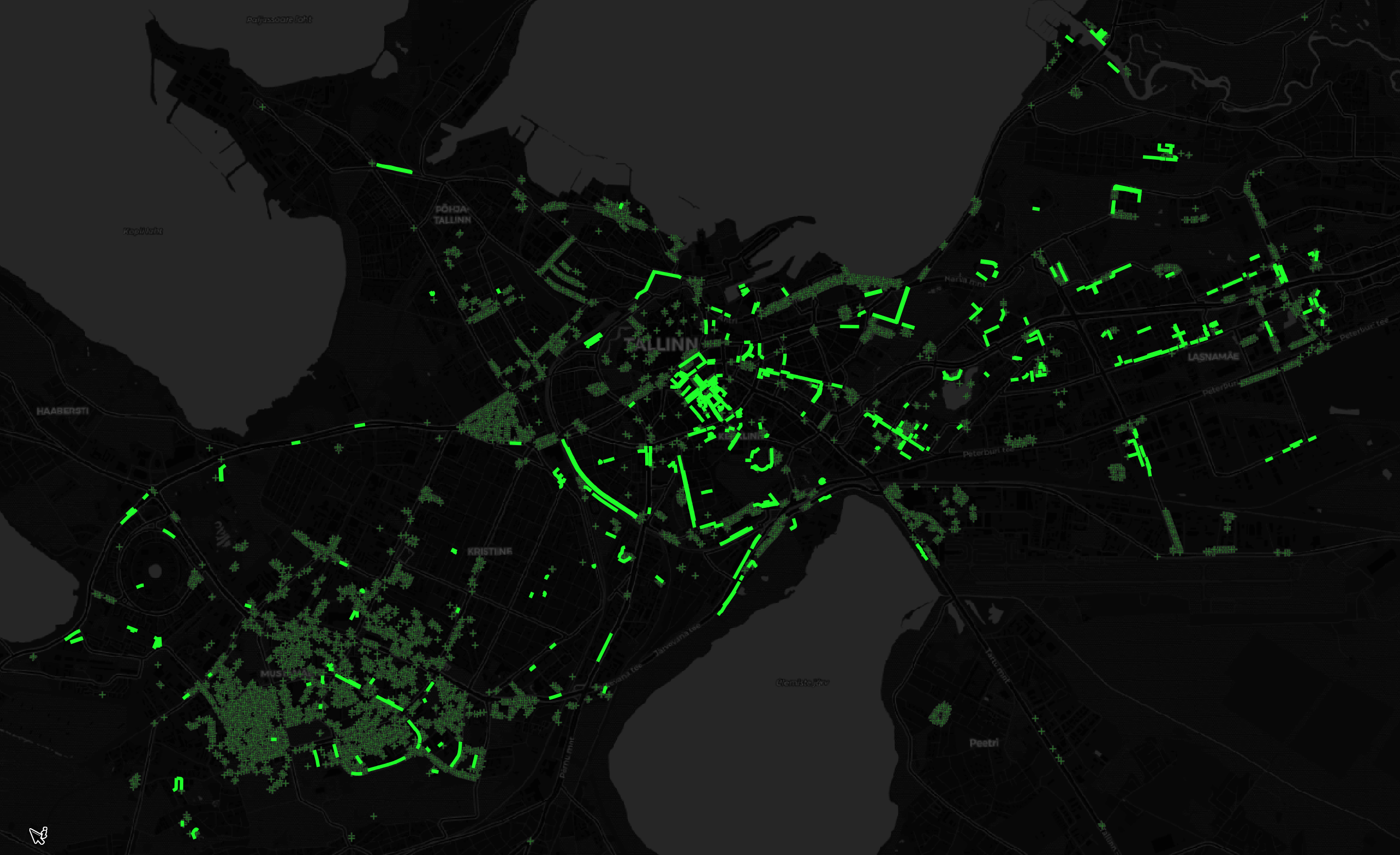
This is what the Estonian Land Board's road data looks like for comparison. The roads are coloured based on how long since their record was last updated.
Every record has been refreshed within the past seven years.
The missing metadata is strange because OSM data for Estonia is generally excellent. I did a quick export of the central business distinct in Tallinn from OSM's site and all the road names appear without issue.
I'll have to revisit this at a later date as there could be a problem with the way I've extracted the street names.
Overture's Land Use Dataset
There are 54 classes within the Tallinn extract I produced, here are the top 15.
SELECT   class,
         COUNT(*)
FROM     tallinn
WHERE    "type" = 'landuse'
GROUP BY 1
ORDER BY 2 DESC
LIMIT    15;
┌─────────────────────────┬──────────────┐
│          class          │ count_star() │
│         varchar         │    int64     │
├─────────────────────────┼──────────────┤
│ grass                   │         8684 │
│ playground              │          567 │
│ residential             │          493 │
│ pitch                   │          433 │
│ forest                  │          310 │
│ pier                    │          306 │
│ garden                  │          216 │
│ park                    │          178 │
│ commercial              │          147 │
│ industrial              │          135 │
│ track                   │           93 │
│ school                  │           80 │
│ retail                  │           67 │
│ construction            │           52 │
│ greenhouse_horticulture │           37 │
├─────────────────────────┴──────────────┤
│ 15 rows                      2 columns │
└────────────────────────────────────────┘
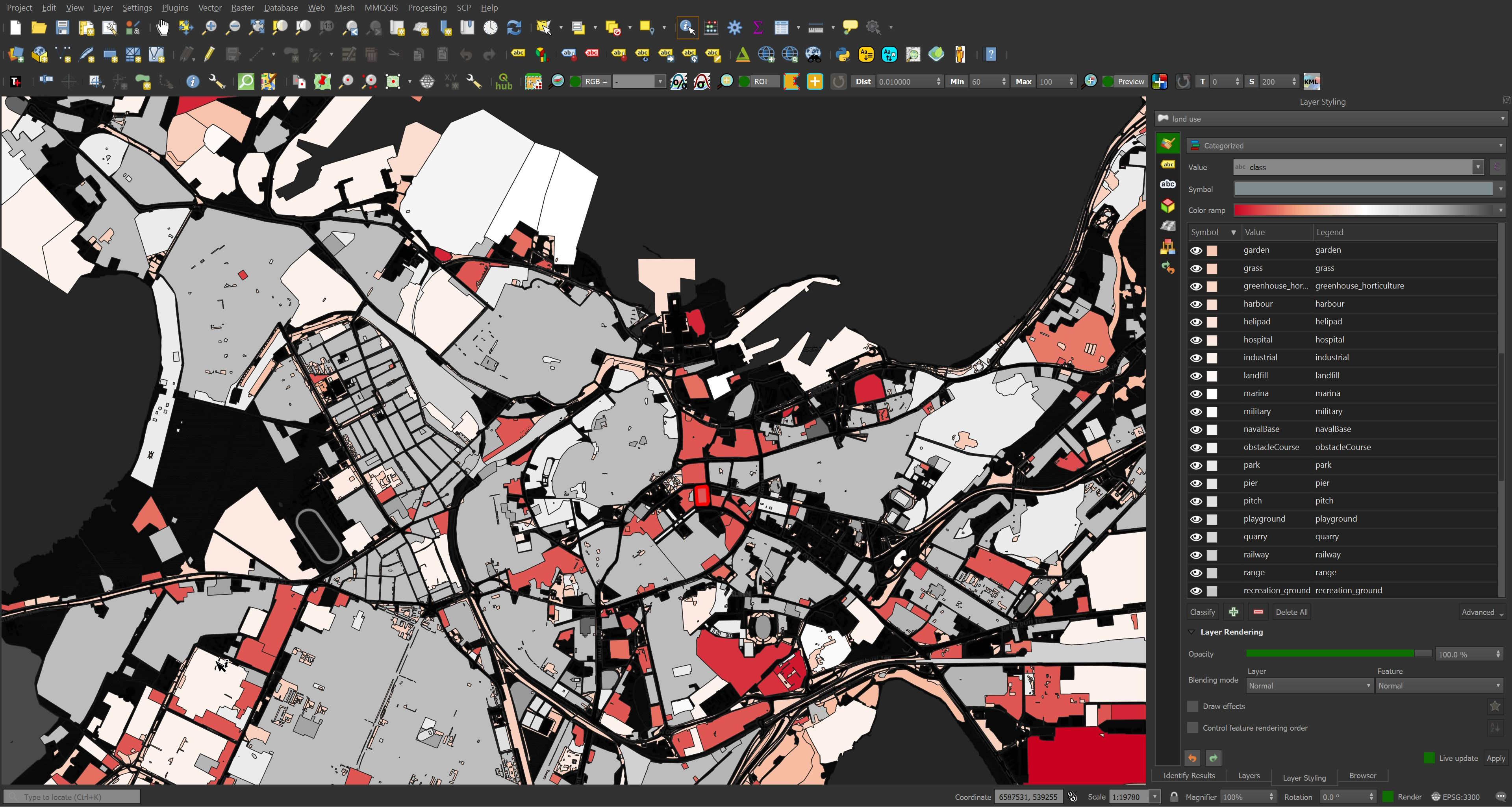
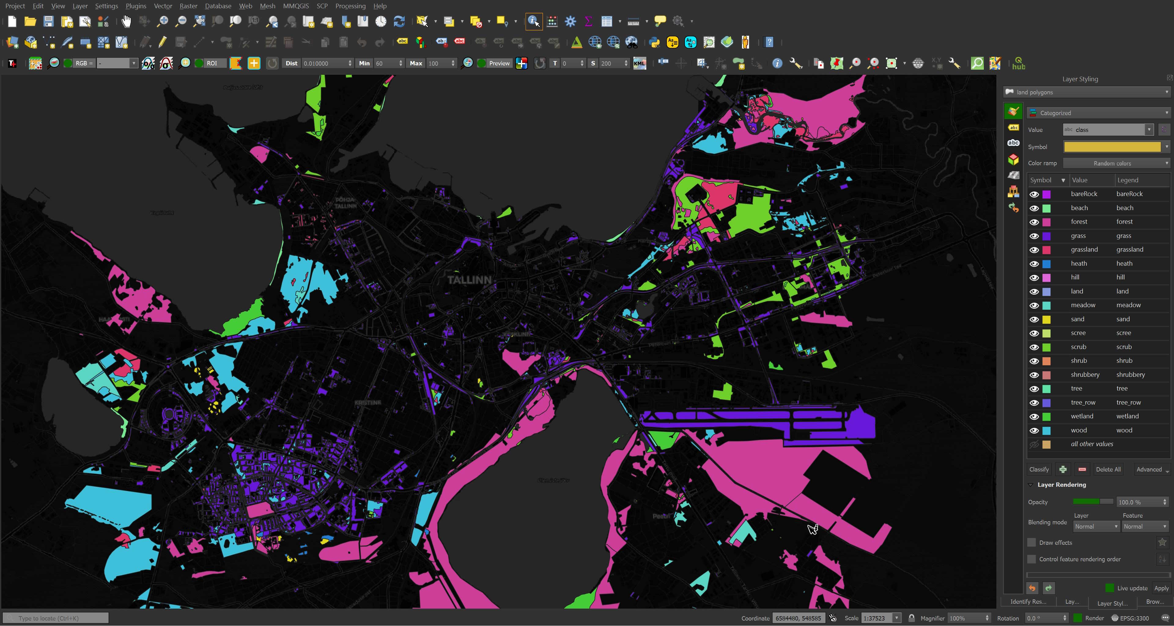
Below are the polygons coloured by their land use class.
There are 18 unique sub-types within the extract.
SELECT   subType,
         COUNT(*)
FROM     tallinn
WHERE    "type" = 'landuse'
GROUP BY 1
ORDER BY 2 DESC;
┌────────────────────┬──────────────┐
│      subType       │ count_star() │
│      varchar       │    int64     │
├────────────────────┼──────────────┤
│ park               │         8863 │
│ recreation         │         1109 │
│ residential        │          522 │
│ developed          │          359 │
│ protected          │          310 │
│ structure          │          306 │
│ horticulture       │          285 │
│ education          │           94 │
│ construction       │           52 │
│                    │           47 │
│ agriculture        │           33 │
│ military           │           18 │
│ medical            │           18 │
│ cemetery           │            9 │
│ resourceExtraction │            9 │
│ religious          │            3 │
│ airport            │            3 │
│ landfill           │            2 │
│ entertainment      │            1 │
├────────────────────┴──────────────┤
│ 19 rows                 2 columns │
└───────────────────────────────────┘
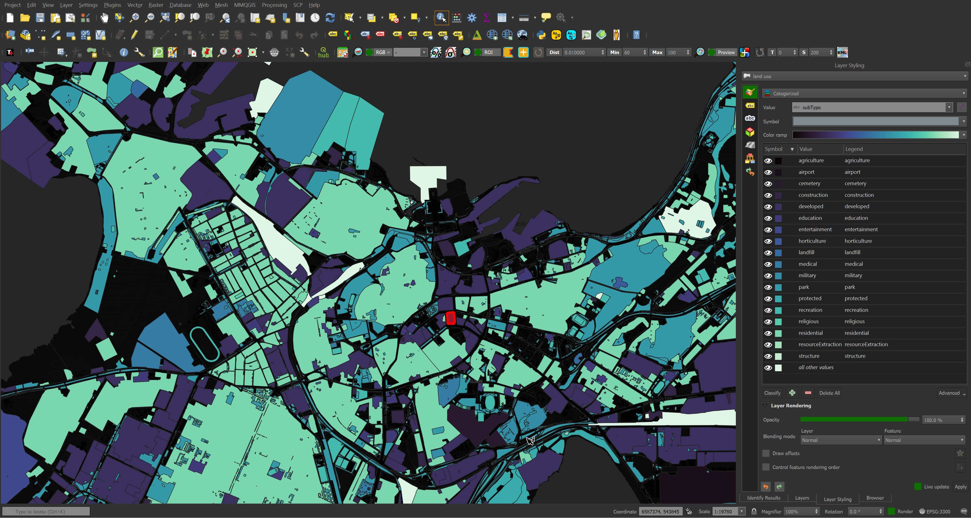
Both of these classifications look very comprehensive and accurate as far as I can tell.
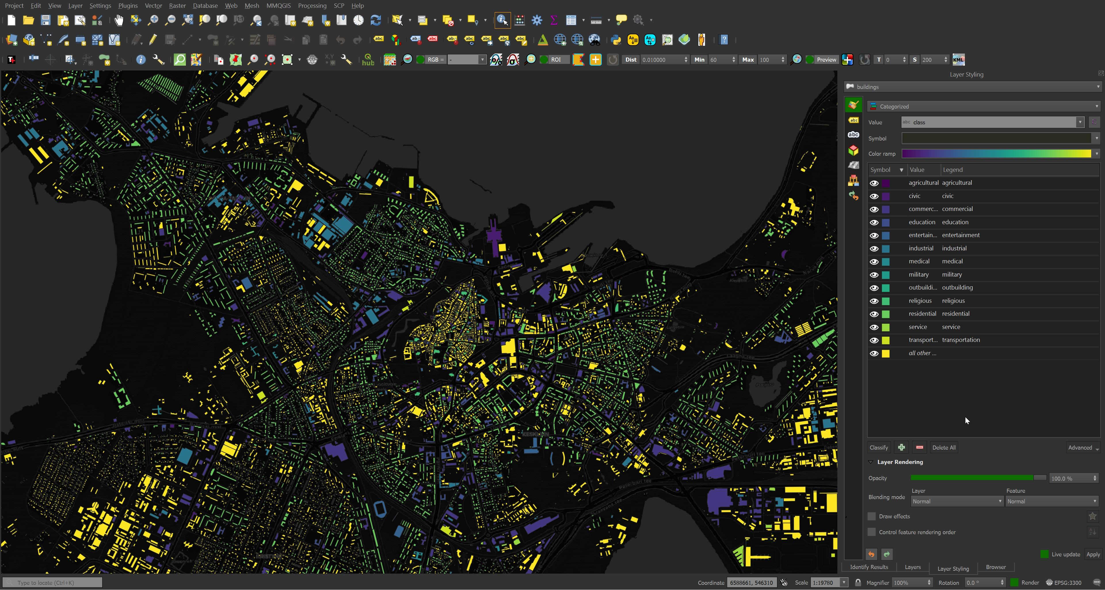
Overture's Buildings Dataset
I can't spot any missing buildings in Overture's Tallinn dataset. The buildings data is sourced from OSM and it looks like every polygon made it over into this release. The class of each building looks comprehensive and accurate as well.
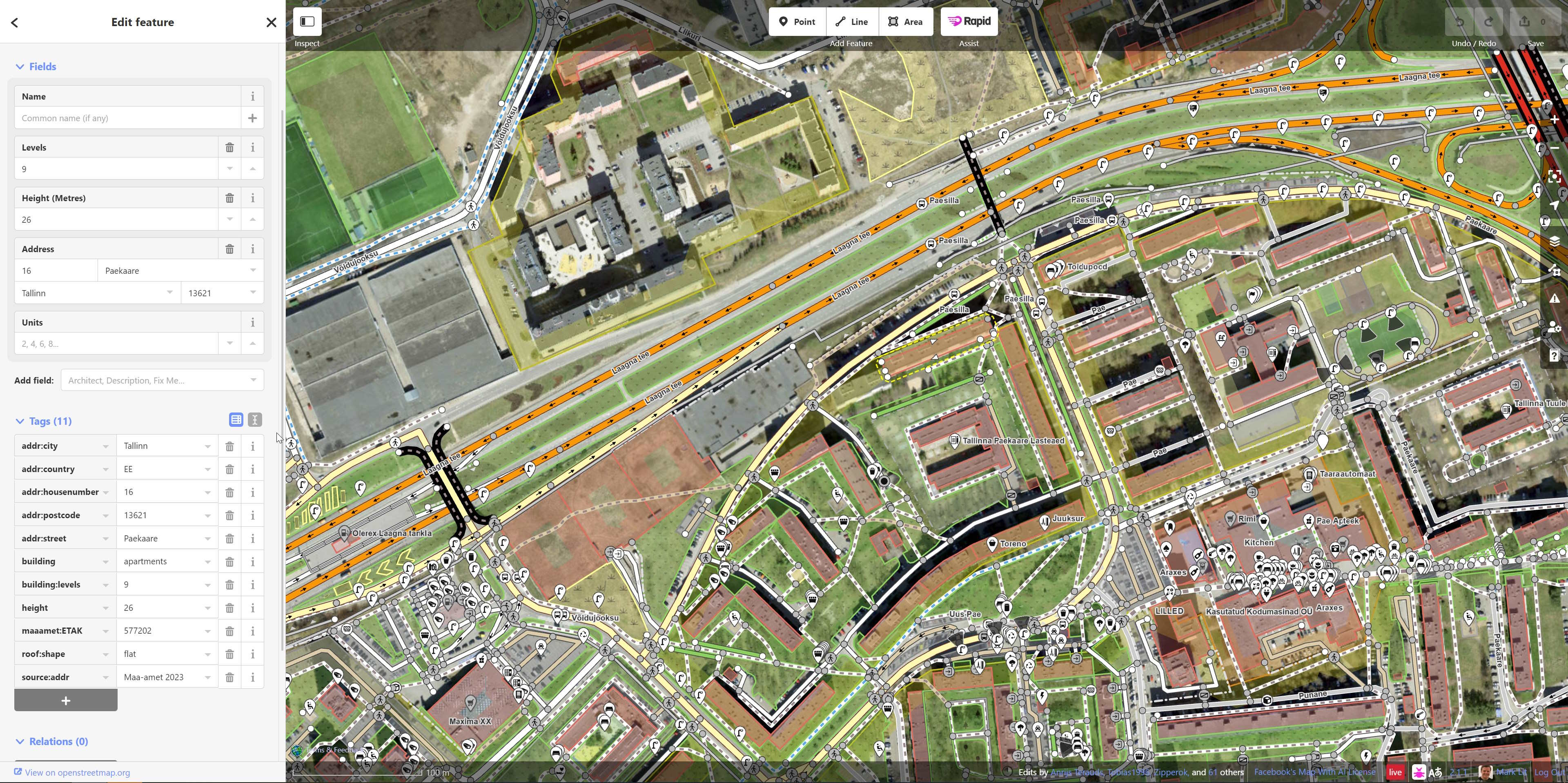
There's floor count data for around ~10% of the buildings in Tallinn. I've highlighted those buildings below.
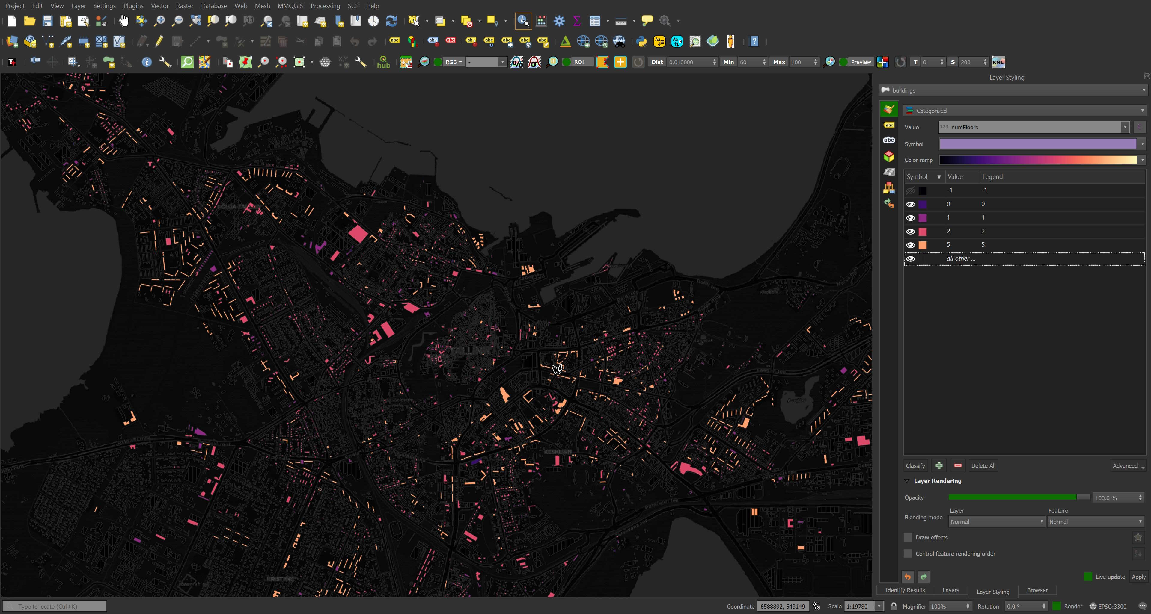
Some neighbourhoods have more floor and height details. This area is full of apartment towers and large retail outlets. Around 25% of the buildings have height information.
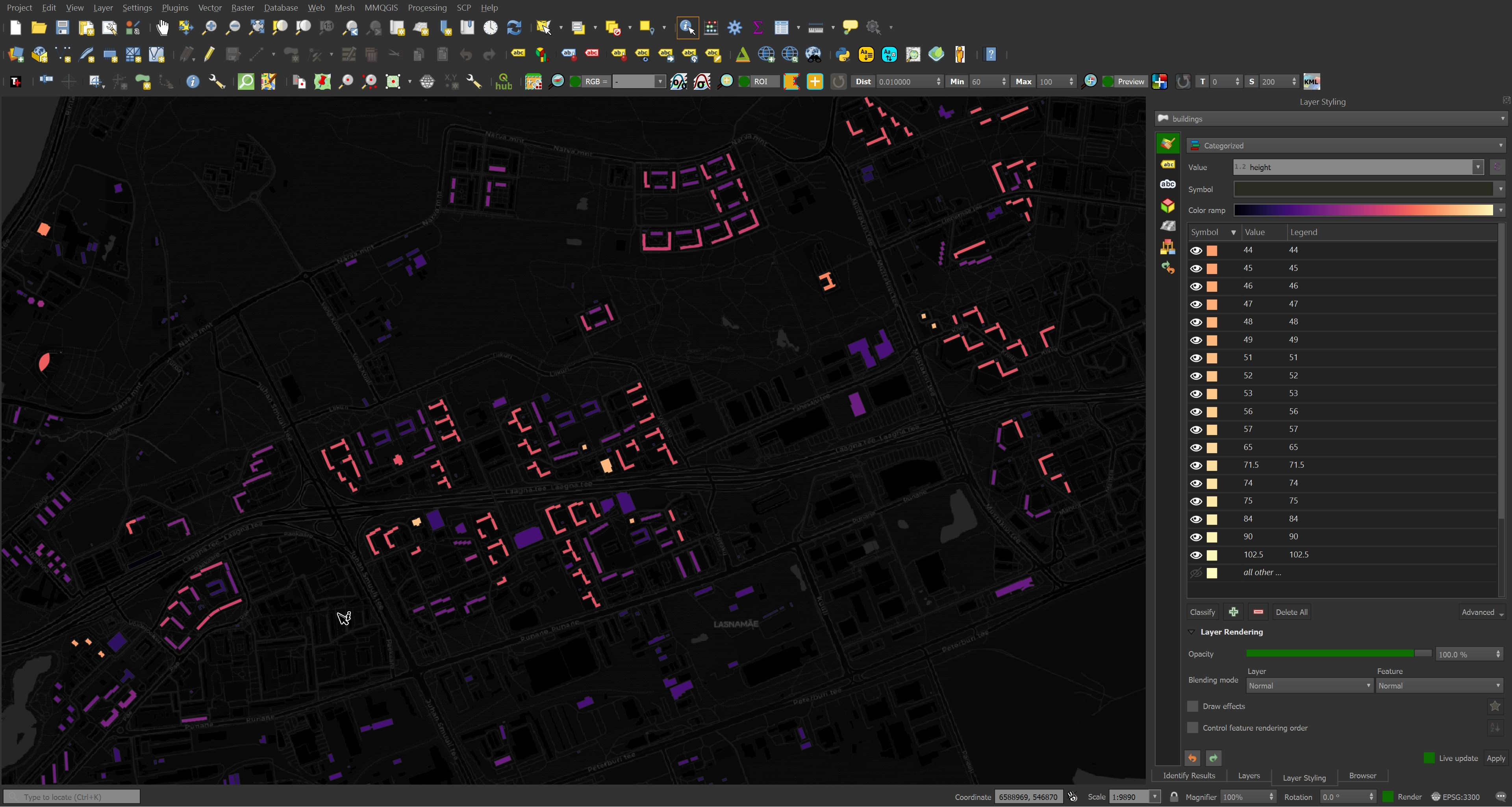
I checked Meta's OSM editor Rapid and floor count as well as overall height are very prominent in the metadata list.
The Estonian Land Board has published vast LiDAR and 3D building datasets. This needs to make its way into OSM in a way the community would accept or become a source for Overture somehow. Governments producing and publishing data in isolation of one another just creates a lot of friction in producing non-hyper-localised GIS products.
Overture's Land Dataset
The points and line strings in my extract were made up of trees and tree lines.
SELECT   subType,
         COUNT(*)
FROM     tallinn
WHERE    "type" = 'land'
AND      ST_GEOMETRYTYPE(geom) = 'POINT'
GROUP BY 1
ORDER BY 2 DESC;
┌──────────┬──────────────┐
│ subType  │ count_star() │
│ varchar  │    int64     │
├──────────┼──────────────┤
│ tree     │        12037 │
│ shrub    │            1 │
│ physical │            1 │
└──────────┴──────────────┘
SELECT   subType,
         COUNT(*)
FROM     tallinn
WHERE    "type" = 'land'
AND      ST_GEOMETRYTYPE(geom) = 'LINESTRING'
GROUP BY 1
ORDER BY 2 DESC;
┌──────────┬──────────────┐
│  class   │ count_star() │
│ varchar  │    int64     │
├──────────┼──────────────┤
│ tree_row │          573 │
└──────────┴──────────────┘
Below is a rendering of the above two geometry types.
The polygons were made up of 15 different land types.
SELECT   subType,
         COUNT(*)
FROM     tallinn
WHERE    "type" = 'land'
AND      ST_GEOMETRYTYPE(geom) LIKE '%POLYGON'
GROUP BY 1
ORDER BY 2 DESC;
┌───────────┬──────────────┐
│   class   │ count_star() │
│  varchar  │    int64     │
├───────────┼──────────────┤
│ grass     │         8723 │
│ wood      │          507 │
│ forest    │          298 │
│ scrub     │          276 │
│ grassland │          234 │
│ sand      │          103 │
│ wetland   │           51 │
│ land      │           32 │
│ meadow    │           29 │
│ heath     │           25 │
│ beach     │           17 │
│ bareRock  │           15 │
│ shrubbery │            2 │
│ tree_row  │            2 │
│ scree     │            1 │
├───────────┴──────────────┤
│ 15 rows        2 columns │
└──────────────────────────┘
I used the following filter in QGIS to remove any land records that were simply classed as "land". There were 32 of these records and they were large squares covering other records.
"type" = 'land' and "class" != 'land'
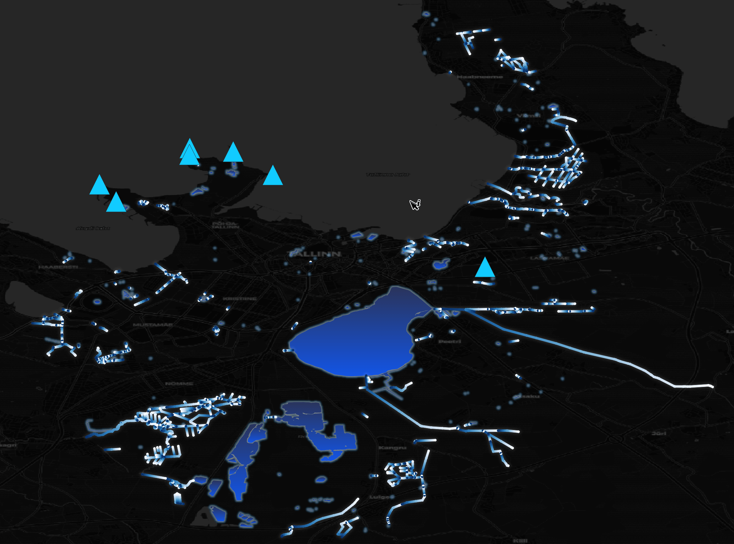
Overture's Water Dataset
There are points, line strings and polygons in the water dataset in the extract I produced. The data is from OSM and looks accurate as far as I can eyeball.
The points are capes, a dock and a swimming pool.
SELECT   subType,
         class,
         type,
         geom
FROM     tallinn
WHERE    "type" = 'water'
AND      ST_GEOMETRYTYPE(geom) = 'POINT'
ORDER BY 2;
┌───────────┬──────────────┬─────────┬───────────────────────────────┐
│  subType  │    class     │  type   │             geom              │
│  varchar  │   varchar    │ varchar │           geometry            │
├───────────┼──────────────┼─────────┼───────────────────────────────┤
│ physical  │ cape         │ water   │ POINT (24.7085738 59.4837611) │
│ physical  │ cape         │ water   │ POINT (24.6888113 59.4852729) │
│ physical  │ cape         │ water   │ POINT (24.6477487 59.4689294) │
│ physical  │ cape         │ water   │ POINT (24.7264963 59.4731469) │
│ physical  │ cape         │ water   │ POINT (24.688582 59.4823844)  │
│ water     │ dock         │ water   │ POINT (24.6552268 59.4610226) │
│ humanMade │ swimmingPool │ water   │ POINT (24.8230303 59.4313317) │
└───────────┴──────────────┴─────────┴───────────────────────────────┘
Overture's Places Datasets
Places is the only dataset that has not used OSM at least partly as a source. Everything in here came from either Microsoft or Meta. A bunch of the good metadata is found inside nested structures so traversing these will be key to extracting key details.
There were 674 top-level categories given for the 17,614 places in the data I extracted for Tallinn. Only 1,829 places lacked any sort of category.
SELECT   REPLACE(JSON_EXTRACT(JSON(categories), '/main'),
                 '"',
                 '') main_category,
         COUNT(*) category
FROM     tallinn
WHERE    "type" = 'place'
GROUP BY 1
ORDER BY 2 DESC
LIMIT    20;
┌──────────────────────────────────┬──────────┐
│          main_category           │ category │
│             varchar              │  int64   │
├──────────────────────────────────┼──────────┤
│                                  │     1829 │
│ beauty_salon                     │     1120 │
│ professional_services            │      476 │
│ shopping                         │      408 │
│ community_services_non_profits   │      340 │
│ automotive_repair                │      258 │
│ cafe                             │      257 │
│ landmark_and_historical_building │      244 │
│ restaurant                       │      218 │
│ spas                             │      199 │
│ beauty_and_spa                   │      191 │
│ real_estate                      │      188 │
│ furniture_store                  │      183 │
│ school                           │      179 │
│ bar                              │      174 │
│ arts_and_entertainment           │      172 │
│ clothing_store                   │      162 │
│ college_university               │      162 │
│ park                             │      159 │
│ flowers_and_gifts_shop           │      157 │
├──────────────────────────────────┴──────────┤
│ 20 rows                           2 columns │
└─────────────────────────────────────────────┘
There are cases where Microsoft is the sole source of a record but they reference many of their own record identifiers as sources.
.mode json

SELECT UNNEST(sources) source
FROM   tallinn
WHERE  "type" = 'place'
AND    LEN(sources) > 3
AND    sources LIKE '%1688849865584228%';
[{"source":"{'property': , 'dataset': msft, 'recordId': 1688849865584288, 'confidence': NULL}"},
 {"source":"{'property': /properties/existence, 'dataset': msft, 'recordId': 1688849865584228, 'confidence': NULL}"},
 {"source":"{'property': /properties/existence, 'dataset': msft, 'recordId': 1688849865584215, 'confidence': NULL}"},
 {"source":"{'property': /properties/existence, 'dataset': msft, 'recordId': 1688849865584196, 'confidence': NULL}"},
 {"source":"{'property': /properties/existence, 'dataset': msft, 'recordId': 1688849865584181, 'confidence': NULL}"},
 {"source":"{'property': /properties/existence, 'dataset': msft, 'recordId': 1688849865584172, 'confidence': NULL}"},
 {"source":"{'property': /properties/existence, 'dataset': msft, 'recordId': 1688849865584145, 'confidence': NULL}"},
 {"source":"{'property': /properties/existence, 'dataset': msft, 'recordId': 1688849865584138, 'confidence': NULL}"},
 {"source":"{'property': /properties/existence, 'dataset': msft, 'recordId': 1688849865584126, 'confidence': NULL}"},
 {"source":"{'property': /properties/existence, 'dataset': msft, 'recordId': 1688849865584117, 'confidence': NULL}"},
 {"source":"{'property': /properties/existence, 'dataset': msft, 'recordId': 1688849865584086, 'confidence': NULL}"}]
Below is a record solely sourced from Microsoft. I've excluded any NULL columns for readability.
.mode json

SELECT addresses,
       bbox,
       brand,
       categories,
       confidence,
       filename,
       geom,
       id,
       names,
       phones,
       sources,
       "type",
       updateTime,
       version,
       websites
FROM   tallinn
WHERE  "type" = 'place'
AND    sources  LIKE '%msft%'
AND    websites LIKE '%coop%'
LIMIT  1;
[
  {
    "addresses": "[{'freeform': Rohuneeme tee 32, 'locality': Viimsi, 'postCode': NULL, 'region': 37, 'country': EE}]",
    "bbox": "{'minx': 24.8199894, 'maxx': 24.8199894, 'miny': 59.5129751, 'maxy': 59.5129751}",
    "brand": "{'names': {'common': NULL, 'official': NULL, 'alternate': NULL, 'short': NULL}, 'wikidata': NULL}",
    "categories": "{'main': NULL, 'alternate': NULL}",
    "confidence": 0.6,
    "filename": "theme=places/type=place/part-02389-87dd7d19-acc8-4d4f-a5ba-20b407a79638.c000.zstd.parquet",
    "geom": "POINT (24.8199894 59.5129751)",
    "id": "562949963889306",
    "names": "{'common': [{'value': Haabneeme Konsum, 'language': et}], 'official': NULL, 'alternate': NULL, 'short': NULL}",
    "phones": "[57438594]",
    "sources": "[{'property': , 'dataset': msft, 'recordId': 562949963889306, 'confidence': NULL}]",
    "type": "place",
    "updateTime": "2023-10-10T00:00:00.000",
    "version": 0,
    "websites": "[https://www.coop.ee/haabneeme-konsum]"
  }
]
Below is a record solely sourced from Meta. Again, I've removed any NULL columns for readability.
.mode json

SELECT addresses,
       bbox,
       brand,
       categories,
       confidence,
       filename,
       geom,
       id,
       names,
       socials,
       sources,
       "type",
       updateTime,
       version,
       websites
FROM   tallinn
WHERE  "type" = 'place'
AND    sources  LIKE '%meta%'
AND    websites LIKE '%viimsiartium%'
LIMIT  1;
[
  {
    "addresses": "[{'freeform': Randvere tee 28, 'locality': Viimsi, 'postCode': NULL, 'region': NULL, 'country': EE}]",
    "bbox": "{'minx': 24.837433, 'maxx': 24.837433, 'miny': 59.5136611, 'maxy': 59.5136611}",
    "brand": "{'names': {'common': NULL, 'official': NULL, 'alternate': NULL, 'short': NULL}, 'wikidata': NULL}",
    "categories": "{'main': cultural_center, 'alternate': [theatre, topic_concert_venue]}",
    "confidence": 0.9317851066589355,
    "filename": "theme=places/type=place/part-02389-87dd7d19-acc8-4d4f-a5ba-20b407a79638.c000.zstd.parquet",
    "geom": "POINT (24.837433 59.5136611)",
    "id": "109392131245437",
    "names": "{'common': [{'value': Viimsi Artium, 'language': local}], 'official': NULL, 'alternate': NULL, 'short': NULL}",
    "socials": "[https://www.facebook.com/109392131245437]",
    "sources": "[{'property': , 'dataset': meta, 'recordId': 109392131245437, 'confidence': NULL}, {'property': /properties/existence, 'dataset': meta, 'recordId': 232201822120185, 'confidence': NULL}]",
    "type": "place",
    "updateTime": "2023-10-10T00:00:00.000",
    "version": 0,
    "websites": "[http://www.viimsiartium.ee]"
  }
]
DuckDB's Spatial extension can export data into GeoPackage format, which is one of the most performant file formats in QGIS. Unfortunately, I found it really slow during the exercise so instead, I'll export a 10% sampling of places to a CSV first and then use GDAL to produce a GeoPackage file.
$ ~/duckdb ~/Downloads/places.duckdb
CREATE OR REPLACE TABLE places AS
    SELECT ST_GEOMFROMWKB(geometry) geom
    FROM READ_PARQUET('theme=places/type=place/part*.zstd.parquet',
                      filename=true,
                      hive_partitioning=1);

COPY (
    SELECT geom as WKT
    FROM   places
    USING SAMPLE 10%
) TO 'places.csv'
  WITH (HEADER,
        FORCE_QUOTE WKT);
When passing a single-column CSV to GDAL, make sure the header has a comma at the end.
$ sed -i '1 s|$|,|' places.csv
The following produced a 377 MB GeoPackage file.
$ ogr2ogr \
    -f GPKG \
    places.gpkg \
    CSV:places.csv \
    -a_srs EPSG:4326
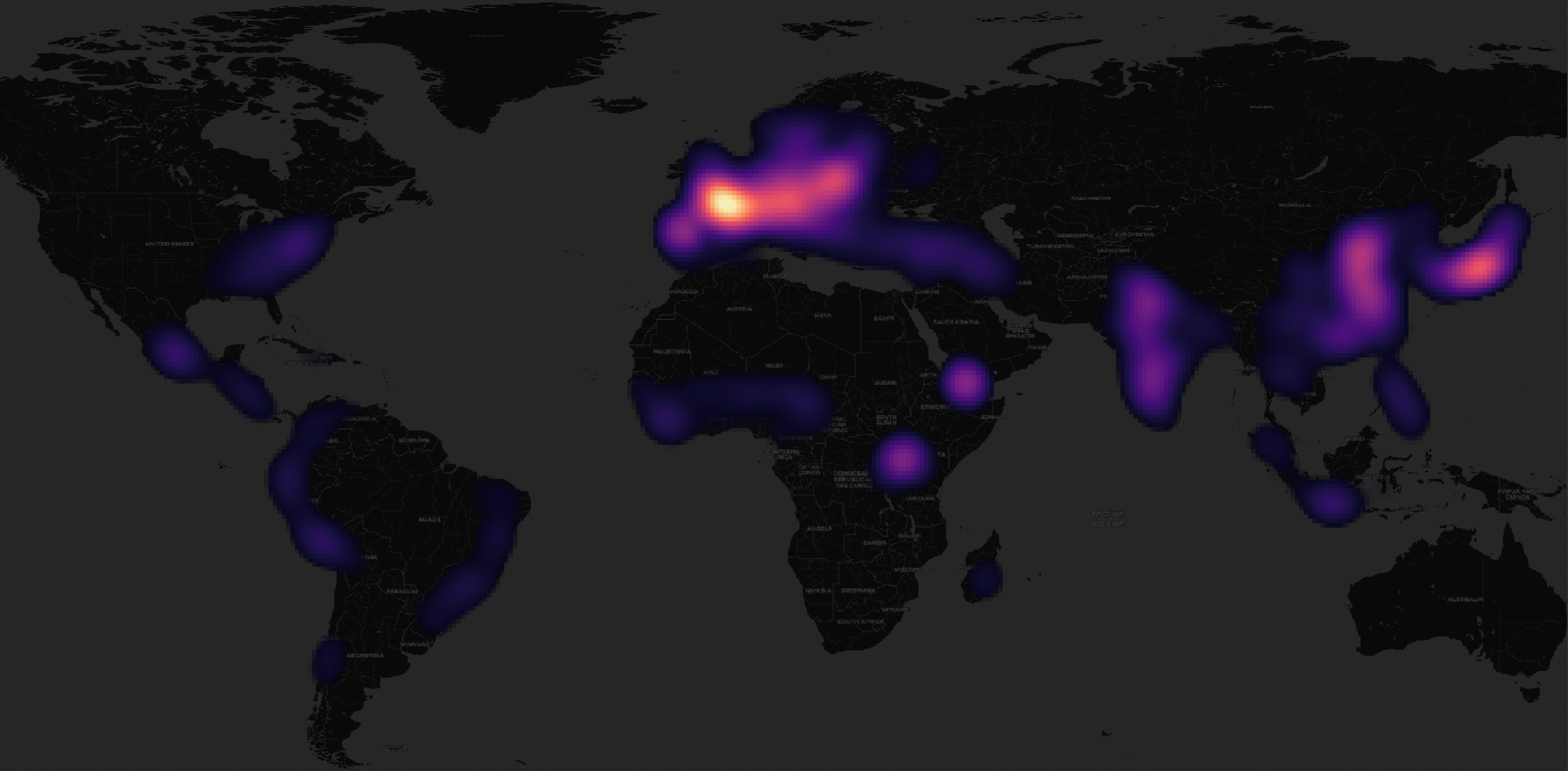
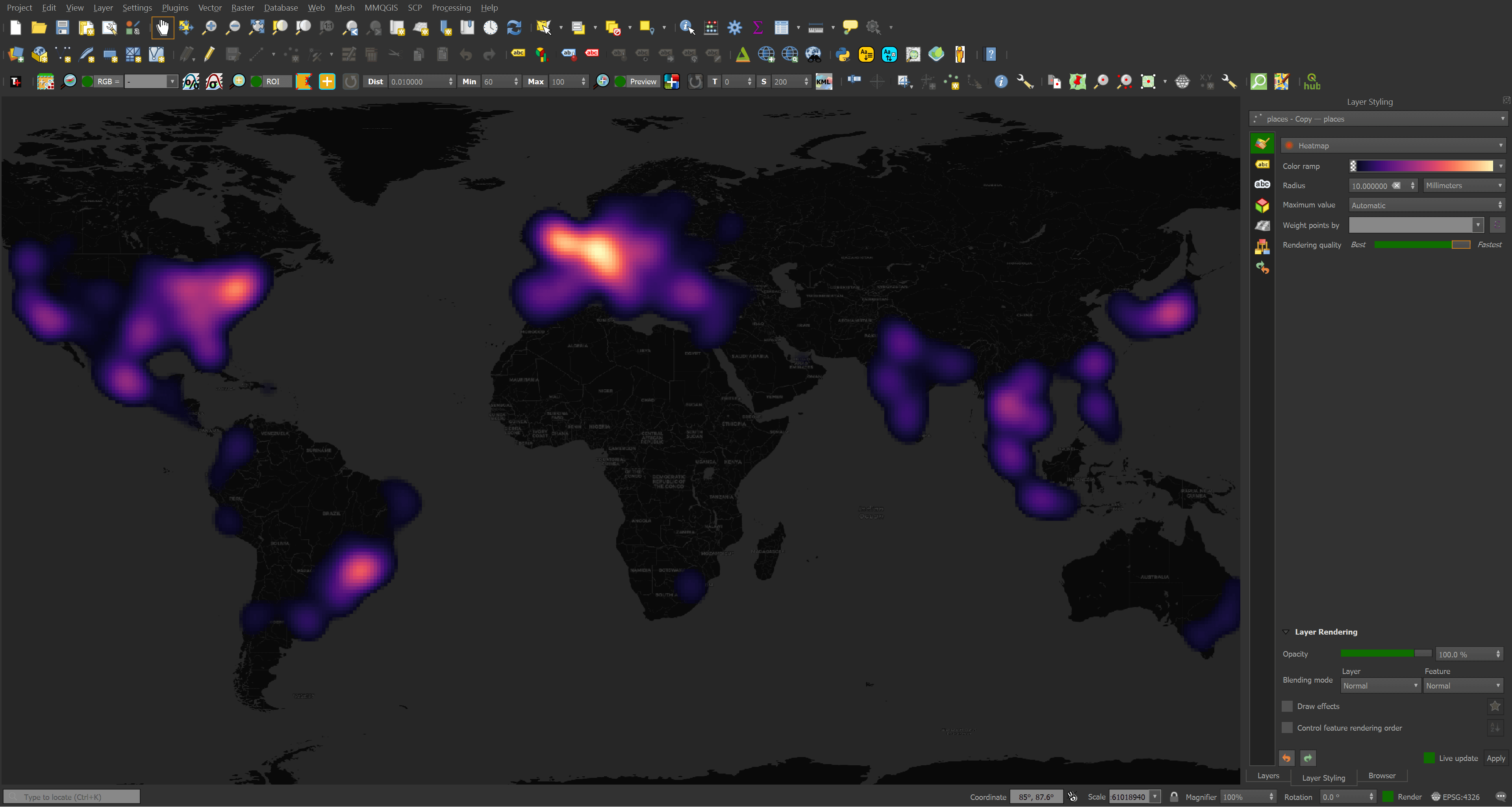
Below shows where the largest clusters of places in Overture's third release are located.
Overture's Administrative Boundaries
The administrative boundaries dataset is made up of 59,281 line strings. Below is a rendering of these coloured based on their administrative level (either 2, 4 or 6). Note these lines are divisions.
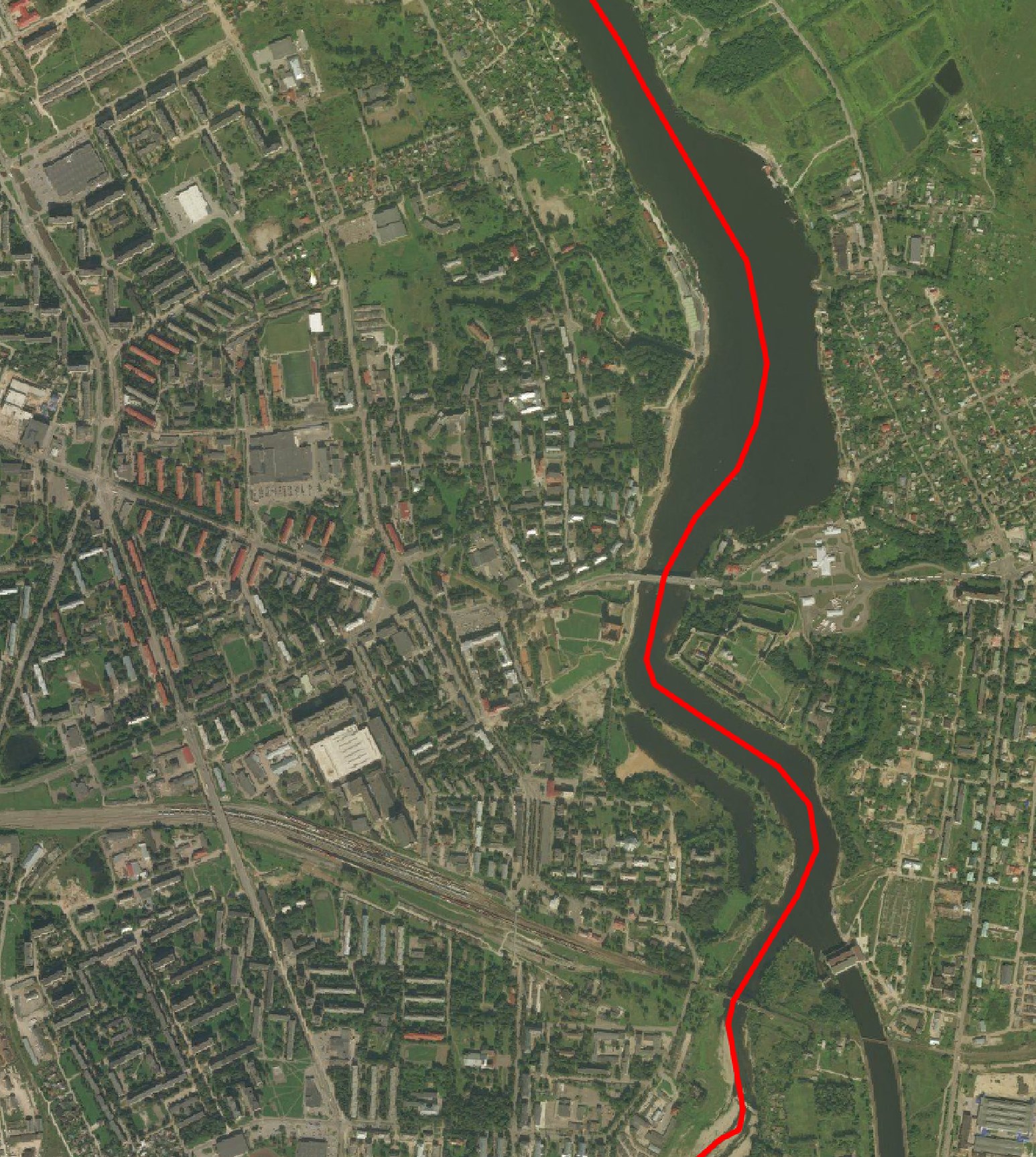
The divisions look to be very detailed and I couldn't spot any issues. Below is the administrative boundary Overture gives for the Estonian-Russian border crossing between Narva and Ivangorod.
Overture's Locality Dataset
There are 3,817,886 records in this dataset. OSM was the main source with Esri contributing to 3,790 of them.
$ ~/duckdb ~/Downloads/locality.duckdb
CREATE OR REPLACE TABLE locality AS
    SELECT * EXCLUDE (geometry),
           ST_GEOMFROMWKB(geometry) geom
    FROM READ_PARQUET('theme=admins/type=locality/part*.zstd.parquet',
                      filename=true,
                      hive_partitioning=1);
The geometry types are mostly points but there are a fair few polygons and multi-polygons.
SELECT   ST_GeometryType(geom)::TEXT geom_type,
         COUNT(*)
FROM     locality
GROUP BY 1
ORDER BY 2 DESC;
┌──────────────┬──────────────┐
│  geom_type   │ count_star() │
│   varchar    │    int64     │
├──────────────┼──────────────┤
│ POINT        │      3395641 │
│ POLYGON      │       405792 │
│ MULTIPOLYGON │        16453 │
└──────────────┴──────────────┘
There are 14 locality types across five different administrative levels.
SELECT   localityType,
         COUNT(*)
FROM     locality
GROUP BY 1
ORDER BY 2 DESC;
┌──────────────┬──────────────┐
│ localityType │ count_star() │
│   varchar    │    int64     │
├──────────────┼──────────────┤
│ hamlet       │      1535830 │
│ village      │      1363781 │
│ neighborhood │       605479 │
│ suburb       │       139628 │
│ town         │       105697 │
│ county       │        23874 │
│ city         │        16168 │
│ region       │        15785 │
│ borough      │         4214 │
│ state        │         3211 │
│ district     │         2215 │
│ municipality │         1523 │
│ country      │          281 │
│ province     │          200 │
├──────────────┴──────────────┤
│ 14 rows           2 columns │
└─────────────────────────────┘
SELECT   adminLevel,
         COUNT(*)
FROM     locality
GROUP BY 1
ORDER BY 2 DESC;
┌────────────┬──────────────┐
│ adminLevel │ count_star() │
│   int32    │    int64     │
├────────────┼──────────────┤
│          8 │      3039204 │
│         10 │       749770 │
│          6 │        24893 │
│          4 │         3738 │
│          2 │          281 │
└────────────┴──────────────┘
I'll dump out a few fields of interest to a JSONL file to give you an idea of what a record looks like.
COPY (
    SELECT ST_GeometryType(geom) geom_type,
           JSON(names) AS names,
           localityType,
           subType,
           adminLevel,
           REGEXP_EXTRACT(updateTime,
                          '([0-9]{4})')::int updated_year,
           geom
    FROM   locality
) TO 'locality.json';
$ head -n1 locality.json | jq -S .
Below you can see a point representing a Hamlet with its name in multiple languages.
{
  "adminLevel": 8,
  "geom": "POINT (112.91038 40.6156877)",
  "geom_type": "POINT",
  "localityType": "hamlet",
  "names": {
    "alternate": null,
    "common": [
      {
        "language": "zh-HanS",
        "value": "元山子"
      },
      {
        "language": "local",
        "value": "Yuanshanzi"
      },
      {
        "language": "zh",
        "value": "元山子"
      },
      {
        "language": "en",
        "value": "Yuanshanzi"
      },
      {
        "language": "zh-HanT",
        "value": "元山子"
      }
    ],
    "official": null,
    "short": null
  },
  "subType": "namedLocality",
  "updated_year": 2023
}
The points counts aren't as dense in as many parts of the world as I would have expected.