Reading H3s like IPs

The hexadecimal form of an H3 index has human-readable elements sort of like how the IPv4 A.B.C.D notation has. The zoom level, region of the world and position from North to South can be figured out from the first four hexadecimal characters.

The second hexadecimal character maps to one of 16 zoom levels. Also, the more zoomed out you are the more Fs will appear at the end.

$ for ZOOM in {0..15}; do
      echo `~/Downloads/h3/build/bin/latLngToCell \
              --latitude 59.44 \
              --longitude 24.75 \
              --resolution $ZOOM`, \
           $ZOOM
  done

8009fffffffffff, 0
8108bffffffffff, 1
82089ffffffffff, 2
83089bfffffffff, 3
84089b1ffffffff, 4
85089b1bfffffff, 5
86089b1a7ffffff, 6
87089b1a2ffffff, 7
88089b1a2bfffff, 8
89089b1a2bbffff, 9
8a089b1a2bb7fff, 10
8b089b1a2bb5fff, 11
8c089b1a2bb53ff, 12
8d089b1a2bb523f, 13
8e089b1a2bb520f, 14
8f089b1a2bb520a, 15

In the continental US at zoom level 7, often H3s start with either 872 or 874. This is handy to remember because if longitude and latitude have been mixed up generating an H3, the 872 or 874 prefix won't be there.

This has the latitude and longitude mixed up for a point in Southern California.

$ ~/Downloads/h3/build/bin/latLngToCell \
        --latitude -118.2173364310 \
        --longitude 33.8939267068 \
        --resolution 7

The resulting H3 starts with an 87e, which is the first hint this isn't in the continental US and something isn't right.

87e30d28effffff

The following uses the correct values for latitude and longitude and produces a value that starts with 872.

$ ~/Downloads/h3/build/bin/latLngToCell \
        --latitude 33.8939267068 \
        --longitude -118.2173364310 \
        --resolution 7

8729a56f0ffffff

The same goes for Europe with 870, 871 or 873 often being the prefix at zoom level 7.

The third hexadecimal character runs from North to South so it can indicate how far you are from either of the poles or the equator.

Below I've generated H3s for Zoom level 0 for much of the world. I'll save them into a CSV file and render them using QGIS.

$ python3

from h3 import h3_to_geo_boundary as get_poly


def h3_to_wkt(h3_hex:str):
    return 'POLYGON((%s))' % \
               ', '.join(['%f %f' % (lon, lat)
                          for lon, lat in get_poly(h3_hex,
                                                   geo_json=True)])

indices = set()

for lon in range(-140, 140):
    for lat in range(-60, 60):
        indices.add(h3.geo_to_h3(lat, lon, 0))

with open('h3_0.csv', 'w') as f:
    f.write('h3,geom\n')

    for index in indices:
        f.write('%s,"%s"\n' % (index, h3_to_wkt(index)))

I've used the first four hexadecimal characters of each H3 for their respective label. The fourth hexadecimal character was used in a colour ramp for the background colour of each polygon.

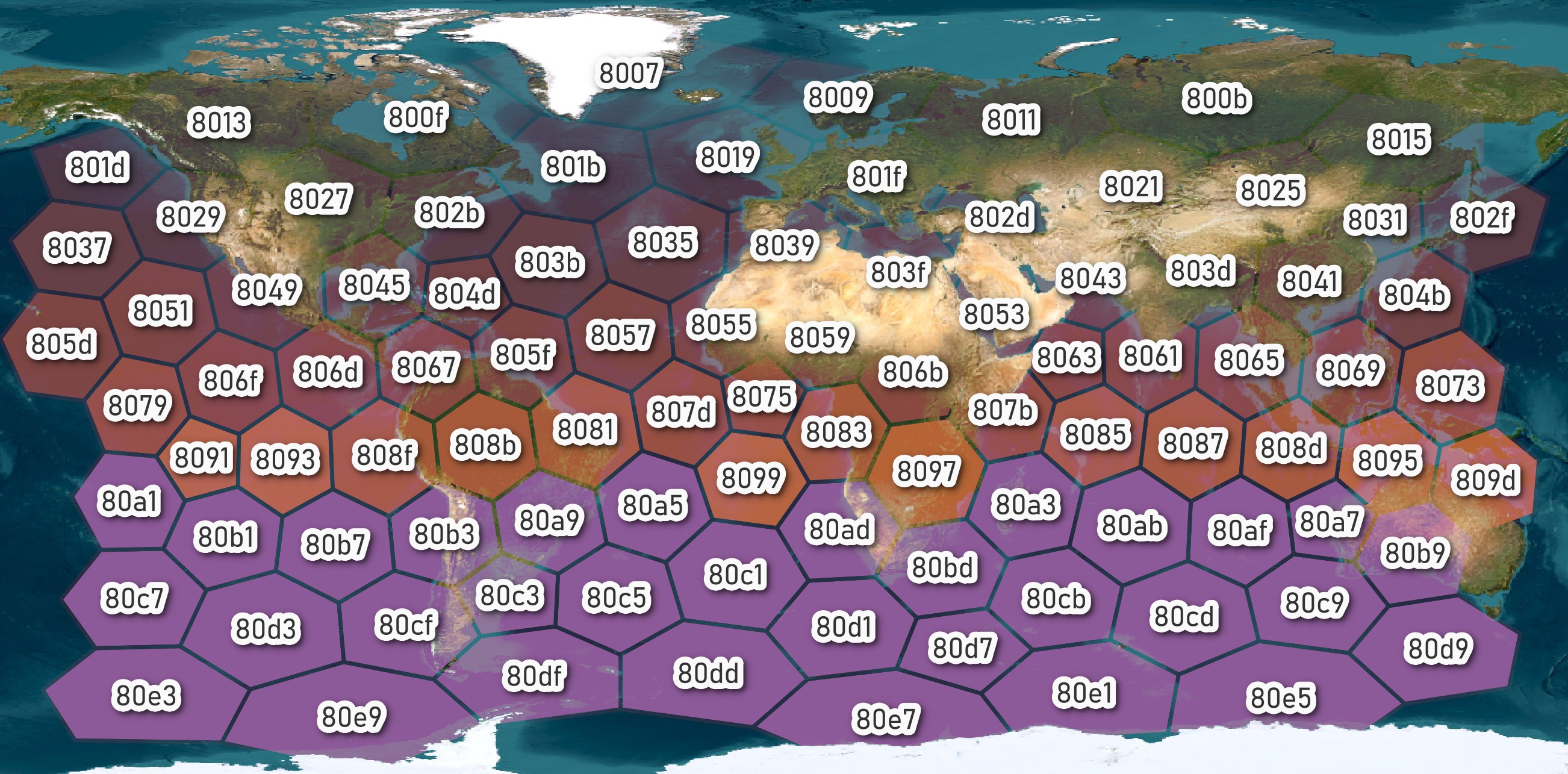
There are a little over one hundred of these 4-character prefixes so memorising them for the regions you commonly work with or even the continent of each isn't too far-fetched.

Neighbouring H3s often share a large portion of their prefixes. If you want to grep out records from a CSV file that neighbour a given H3, you can do so by simply matching on the first few hexadecimal characters.

$ grep '87089b[a-z0-9]{9}' tallinn.csv

DuckDB's H3 Support

The underlying H3 library has been written in C and contains 13,800 lines of code. Over 85% of the repository's contents are dedicated to its test suite. Isaac Brodsky, who worked for Uber between 2015 and 2019, is the top committer to this project. Isaac is still active in creating new database and programming language bindings for H3, including the H3 extension for DuckDB.

This summer, Isaac added support for WKT rendering of H3s using SQL in DuckDB via his extension. In the past, I'd use Python in an intermediate enrichment step to convert H3s into polygons but now I can produce WKTs in DuckDB and export them to CSV files before loading them into QGIS.

.mode csv

SELECT H3_CELL_TO_BOUNDARY_WKT('8f089b1a2bb520a') geom;

geom
"POLYGON ((24.749998 59.440000, 24.750006 59.439998, 24.750013 59.440001, 24.750012 59.440006, 24.750005 59.440008, 24.749998 59.440005, 24.749998 59.440000))"

Thank you very much to Isaac for this patch.

Building the H3 Extension

If you're using a Mac, Homebrew is a fantastic package manager and I'll use it to install the H3 library, Python and some build tools.

$ brew install \
    cmake \
    csvkit \
    git \
    h3 \
    jq \
    ninja \
    openssl@3 \
    virtualenv

On Ubuntu for Windows or Ubuntu 20 LTS, Uber's H3 library requires at a minimum CMake v3.20 and Ubuntu 20 only ships with v3.16. Below I'll build and install version 3.20.

$ sudo apt update
$ sudo apt install \
    build-essential \
    csvkit \
    jq \
    ninja-build \
    python3-pip \
    python3-virtualenv

This builds CMake v3.20.

$ cd ~/Downloads
$ wget -c https://github.com/Kitware/CMake/releases/download/v3.20.0/cmake-3.20.0.tar.gz
$ tar -xzf cmake-3.20.0.tar.gz
$ cd cmake-3.20.0

$ ./bootstrap --parallel=$(nproc)
$ make -j$(nproc)

$ sudo make install

This is the Ubuntu for Windows and Ubuntu 20 LTS-specific build step for the H3 library.

$ cd ~/Downloads
$ git clone https://github.com/uber/h3
$ mkdir -p h3/build
$ cd h3/build

$ cmake ..
$ make -j$(nproc)

$ sudo make install
$ sudo ldconfig

With the above dependencies installed, I'll clone the DuckDB H3 repo which contains a submodule for DuckDB as well. This step is applicable to all platforms.

$ cd ~/Downloads
$ git clone https://github.com/isaacbrodsky/h3-duckdb duckdb_h3
$ cd ./duckdb_h3
$ git submodule update --init

$ GEN=ninja \
    make \
    duckdb_release \
    release

I'll create a Python Virtual Environment that'll be used below.

$ virtualenv ~/.h3
$ source ~/.h3/bin/activate
$ python3 -m pip install h3

QGIS is open source and has pre-compiled binaries available on all major desktop platforms. I'll be using it for the visualisations in this post.

Cell Tower Observations

OpenCelliD is a community project that collects GPS positions and network coverage patterns from cell towers around the globe. They produce a 48M-record dataset that is refreshed daily. This dataset is delivered as a GZIP-compressed CSV file.

I'll enrich its data with a telecoms carrier dataset called 'mcc-mnc-table'.

The following will download both datasets. Please replace the token in the OpenCelliD URL with your own.

$ cd ~/Downloads

$ git clone https://github.com/IlayG01/mcc-mnc-table

$ wget -O cell_towers.csv.gz \
    "https://opencellid.org/ocid/downloads?token=...&type=full&file=cell_towers.csv.gz"

Below is an example record from OpenCelliD.

$ gunzip -c cell_towers.csv.gz \
    | head -n2 \
    | csvjson \
    | jq -S .

[
  {
    "area": 801,
    "averageSignal": false,
    "cell": 86355,
    "changeable": true,
    "created": 1282569574,
    "lat": 52.522202,
    "lon": 13.285512,
    "mcc": 262,
    "net": 2,
    "radio": "UMTS",
    "range": 1000,
    "samples": 7,
    "unit": false,
    "updated": 1300155341
  }
]

Below is an example record from the mcc-mnc-table dataset.

$ jq -S '.[0]' mcc-mnc-table/mcc-mnc-table.json

{
  "country": "Abkhazia",
  "country_code": 7,
  "iso": "ge",
  "mcc": 289,
  "mnc": 88,
  "network": "A-Mobile"
}

H3 Enrichment in DuckDB

The following will import both datasets into DuckDB.

$ ~/Downloads/duckdb_h3/duckdb/build/release/duckdb \
    -unsigned \
    ~/Downloads/opencellid.duckdb

LOAD '/home/mark/Downloads/duckdb_h3/build/release/h3.duckdb_extension';

CREATE OR REPLACE TABLE observations AS
    SELECT * EXCLUDE(created, lat, lon, updated),
        to_timestamp(created) created,
        to_timestamp(updated) updated,
        printf('%x', h3_latlng_to_cell(
                         lat,
                         lon,
                         2)::bigint) as h3_2
    FROM 'cell_towers.csv.gz';

CREATE OR REPLACE TABLE carriers AS
    SELECT *
    FROM read_json_auto('mcc-mnc-table/mcc-mnc-table.json');

I wanted to wrap the following aggregation step inside of the COPY statement below but DuckDB exhausted the 32 GB of RAM available on my system when I tried. I'll create a stats table first to bake in the aggregation and then dump it out with the WKT of each H3s polygon into a CSV file afterward. Breaking this up into two steps is much more RAM-friendly.

CREATE OR REPLACE TABLE stats AS
    SELECT c.network network,
           o.radio radio,
           sum(o.samples) num_samples,
           o.h3_2 h3_2
    FROM observations o
    JOIN carriers c ON (o.mcc = c.mcc)
    GROUP BY 1, 2, 4;

COPY (
    SELECT *,
           H3_CELL_TO_BOUNDARY_WKT(h3_2) geom
    FROM stats
) TO '/home/mark/Downloads/samples_by_h3_0.csv' (HEADER);

A total of 133,950 records were exported. The following is what the first record looks like.

$ head -n2 ~/Downloads/samples_by_h3_0.csv \
    | csvjson \
    | jq -S .

[
  {
    "geom": "POLYGON ((11.080660 61.540515, 10.279089 60.275949, 12.360313 59.444957, 15.277419 59.851205, 16.213285 61.104087, 14.102102 61.963541, 11.080660 61.540515))",
    "h3_2": "8208a7fffffffff",
    "network": "unifon",
    "num_samples": 743166,
    "radio": "GSM"
  }
]

Visualising in QGIS

I'll be using a color ramp called Wiener Challah for these visualisations. Its ZIP file contains a 591-byte XML file that'll be imported into QGIS.

<!DOCTYPE qgis_style>
<qgis_style version="2">
  <symbols/>
  <colorramps>
    <colorramp tags="Colorful" type="gradient" name="Wiener Challah">
      <prop v="63,51,65,255" k="color1"/>
      <prop v="255,244,157,255" k="color2"/>
      <prop v="0" k="discrete"/>
      <prop v="gradient" k="rampType"/>
      <prop v="0.193588;102,65,71,255:0.399507;142,74,63,255:0.604192;192,107,50,255:0.696671;229,137,33,255:0.803946;249,179,44,255:0.9;255,206,88,255" k="stops"/>
    </colorramp>
  </colorramps>
  <textformats/>
  <labelsettings/>
  <legendpatchshapes/>
  <symbols3d/>
</qgis_style>

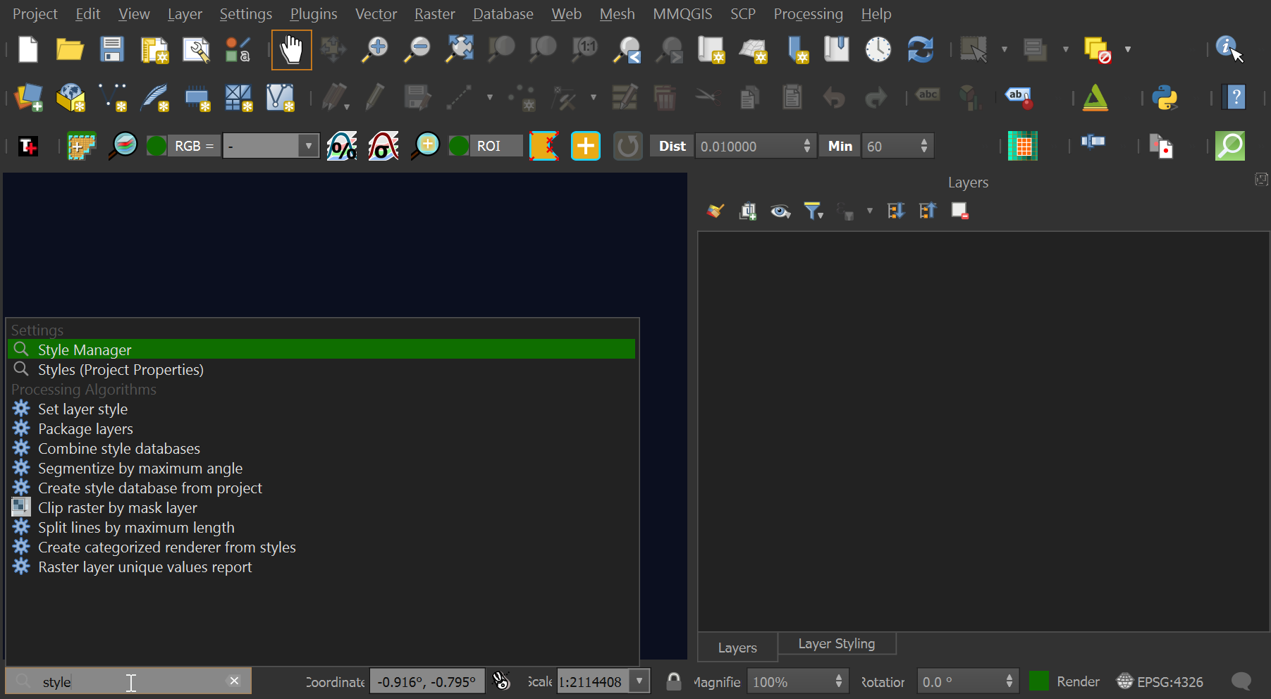
I'll launch QGIS and then start a new project. In the bottom left of the UI, there is a search box. Type in 'Style Manager' and select the first option.

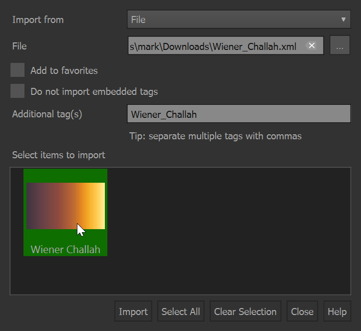
Click 'Import / Export' in the bottom left of the dialog and then 'Import Item(s)'. Select 'Wiener_Challah.xml' which you should extract from the above ZIP file. Click the 'Wiener Challah' gradient and with that selected, click the 'Import' button at the bottom of the dialog. Then click the 'Close' button.

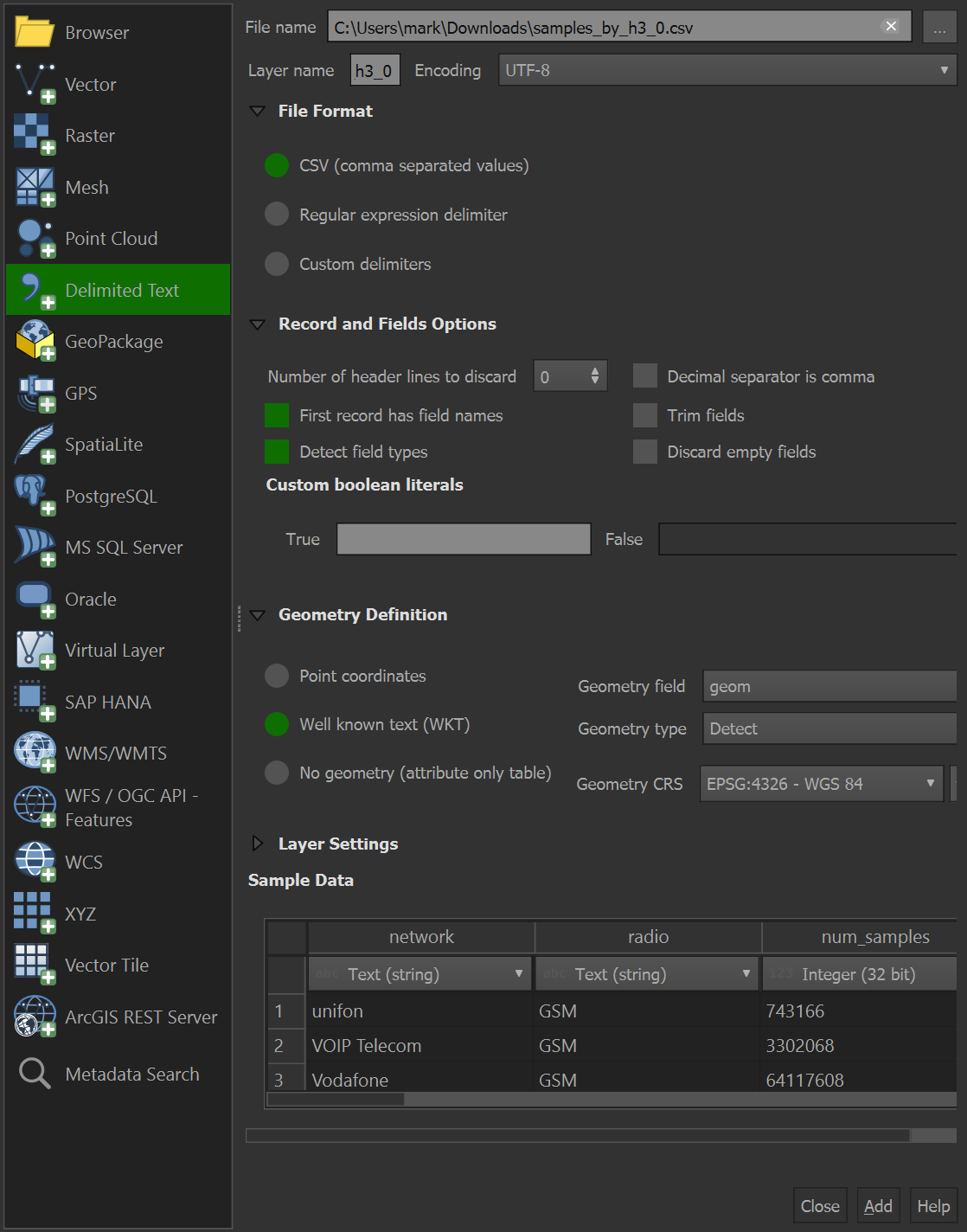
Click the "Layer" Menu -> "Add Layer" -> "Add Delimited Text Layer". Select the samples_by_h3_0.csv file as the file name. Under 'Record and Fields Options' tick the 'First record has field names' box. Under 'Geometry Definition' select 'Well known text (WKT)'. Click the 'Add' button in the bottom right of the dialog and then click the 'Close' button.

If the Layers Panel isn't visible, click the "View" Menu -> "Panels" -> "Layers" and then also click "Layer Styling" as well. You can drag both panels to the right of the UI so at least one is always visible and you can switch between them with the tabs at the bottom of each panel.

The Tile+ plugin for QGIS lets you import satellite and pre-rendered basemaps into QGIS projects. It supports a large number of sources and I'll be using it to fetch satellite imagery. Once it's installed, click the "Plugins" Menu -> "Tile+". Select "Esri World Imagery" from the drop-down and then click the plus button. Make sure this layer is below the 'samples_by_h3_0' layer (the one with the hexagons).

Click the 'samples_by_h3_0' layer. Then the "Layer Styling" tab at the bottom of the panel. Then click 'Simple Fill' under the 'Fill' style item at the top of the panel.

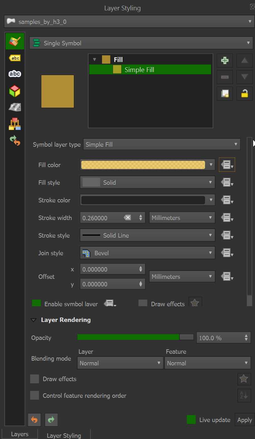
Click the drop-down next to 'Fill color' and select 'Edit'. Paste in the following expression:

ramp_color('Wiener Challah', "num_samples" / 500000)

Right-click the 'samples_by_h3_0' layer and select 'Filter'. Paste the following formula in.

"num_samples" > 10000 and "network" = 'Vodafone' and "radio" = 'UMTS'

Set the Stoke Style to None.

QGIS should resemble the following image.

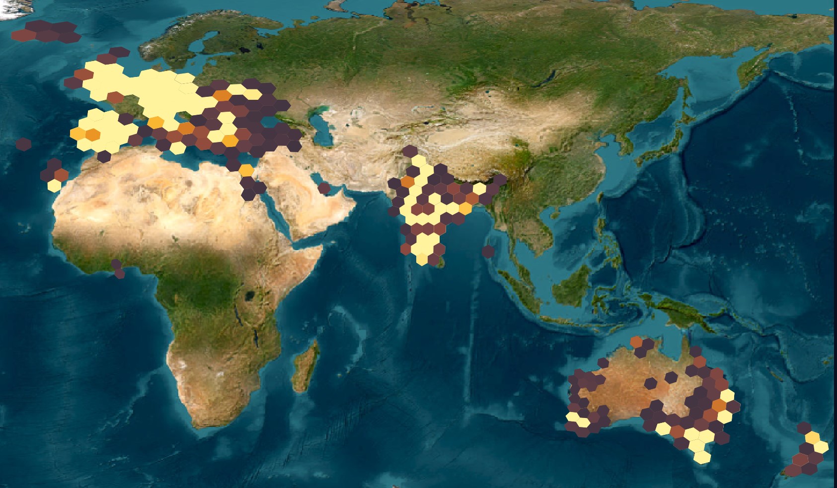
The yellow hexagons represent where the largest number of samples have occurred and these correlate well with population densities in Vodafone's respective markets.

Labels in QGIS

If you want to have labels on each hexagon displaying their sample count then select the 'samples_by_h3_0' layer and then in the "Layer Styling" panel, there is an 'ABC' icon on top of a yellow arrow in the top left which lets you configure Labels. Click on it and make sure the 'Value' drop-down at the top of the panel is set to 'num_samples'.

The 3rd tab from the left underneath that 'Value' drop-down is where you can enable text buffer drawing. The 6th tab from the left lets you configure the drop shadow. These will help contrast the labels to the underlying map and hexagons.

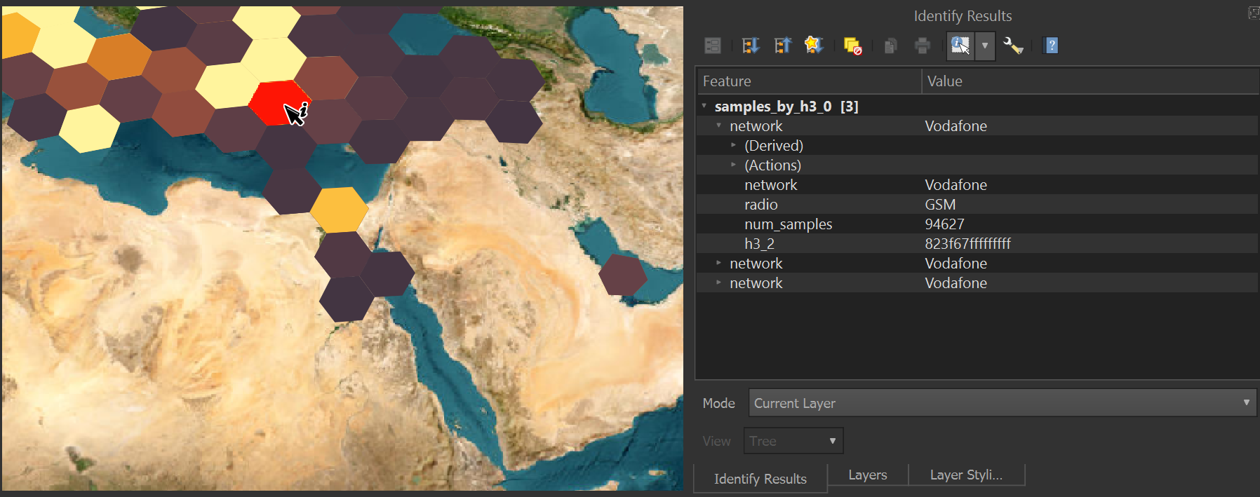
Identifying Features

In the top toolbar of the UI to the right, there is a blue circle with the letter 'i' and a mouse on top of it. This is the 'Identify Features' tool. It'll allow you to click on and/or click-drag over any number of hexagons and bring up a panel with their values. Make sure the 'samples_by_h3_0' layer is selected first before trying to click on any hexagons.