OpenStreetMap (OSM) is the world's largest, most comprehensive, free geographic database. It was founded in the UK in the Summer of 2004 by Steve Coast. Steve has spent his career outside of OSM working for firms such as Grab, Microsoft, Maxar, TomTom and Wolfram Research.
The OSM dataset is consumed by 10s of millions of users and in the past 30 days has received contributions by over 50K individuals producing almost four million changes every day.
Geofabrik, a German-based consulting firm, produces country and region-specific downloads of the OSM dataset that are refreshed every day. One of the file formats used is the Protocol buffer Binary Format (PBF). For a country like Estonia, the PBF file is around 100 MB.
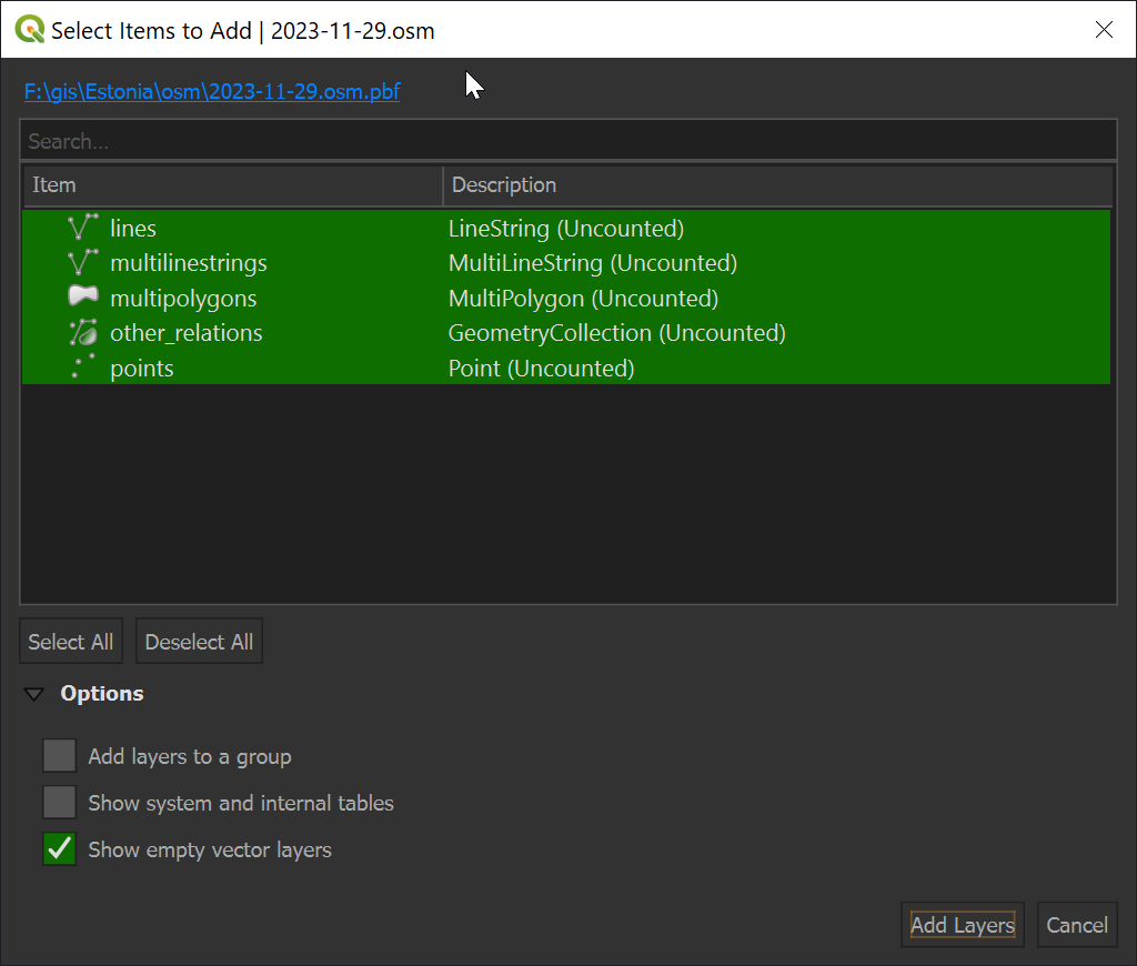
These files can be used, among other applications, to produce maps. The PBF files can be dropped onto QGIS' interface and it'll import the entirety of the dataset into a new scene.
The issue around doing this is that there are 100s of different types of information contained within any one PBF file, even when the geographic area is very narrow. QGIS initially only offers the chance to filter on geometry type when you first drop the PBF file onto its interface.
Any one geometry type could contain hundreds of different types of records. These aren't categorised in a way that is easy to discover and pick apart in QGIS. Below are the multi-polygon records for OSM's Estonia dataset.

The metadata for each record is stored as a plain-text key-value string rather than JSON. Below I'll extract the most common tags used for Estonia's multi-polygon dataset.
$ ~/duckdb
COPY (
    SELECT other_tags
    FROM   ST_READ('2023-11-28.osm.pbf',
                   open_options=['INTERLEAVED_READING=YES'],
                   layer='multipolygons',
                   sequential_layer_scan=true)
) TO '2023-11-28.other_tags.multipolygons.json';
The above extracted 9,632 multi-polygon records. Below are the ten most common other_tag values.
$ sort 2023-11-28.other_tags.json | uniq -c | sort -rn | head
302 {"other_tags":"\"natural\"=>\"water\",\"type\"=>\"multipolygon\""}
262 {"other_tags":"\"landuse\"=>\"farmland\",\"type\"=>\"multipolygon\""}
227 {"other_tags":"\"landuse\"=>\"forest\",\"leaf_type\"=>\"mixed\",\"type\"=>\"multipolygon\""}
168 {"other_tags":"\"landuse\"=>\"meadow\",\"type\"=>\"multipolygon\""}
150 {"other_tags":"\"landuse\"=>\"forest\",\"type\"=>\"multipolygon\""}
147 {"other_tags":"\"natural\"=>\"wood\",\"type\"=>\"multipolygon\""}
135 {"other_tags":"\"landuse\"=>\"grass\",\"type\"=>\"multipolygon\""}
110 {"other_tags":"\"natural\"=>\"scrub\",\"type\"=>\"multipolygon\""}
105 {"other_tags":"\"natural\"=>\"grassland\",\"type\"=>\"multipolygon\""}
105 {"other_tags":"\"landuse\"=>\"forest\",\"leaf_type\"=>\"needleleaved\",\"type\"=>\"multipolygon\""}
You'll end up needing to do a lot of string manipulation to create filters in QGIS to isolate the geometry of interest.
When I was working on my Natural Earth post a few weeks ago, I was taken aback by how convenient it was to have each feature type as its own Shapefile. There was one file for country borders, railroads, time zones, airports, etc.. Each file could be dragged onto QGIS and would render quickly as no one file contained an overwhelming amount of data.
In contrast, when I drop OSM's PBF file for Estonia onto QGIS, my system takes ages to complete the first render. Every action from then on is very sluggish. When using QGIS, you only want to import the absolutely smallest amount of data you can get away with if you want the application to remain responsive.
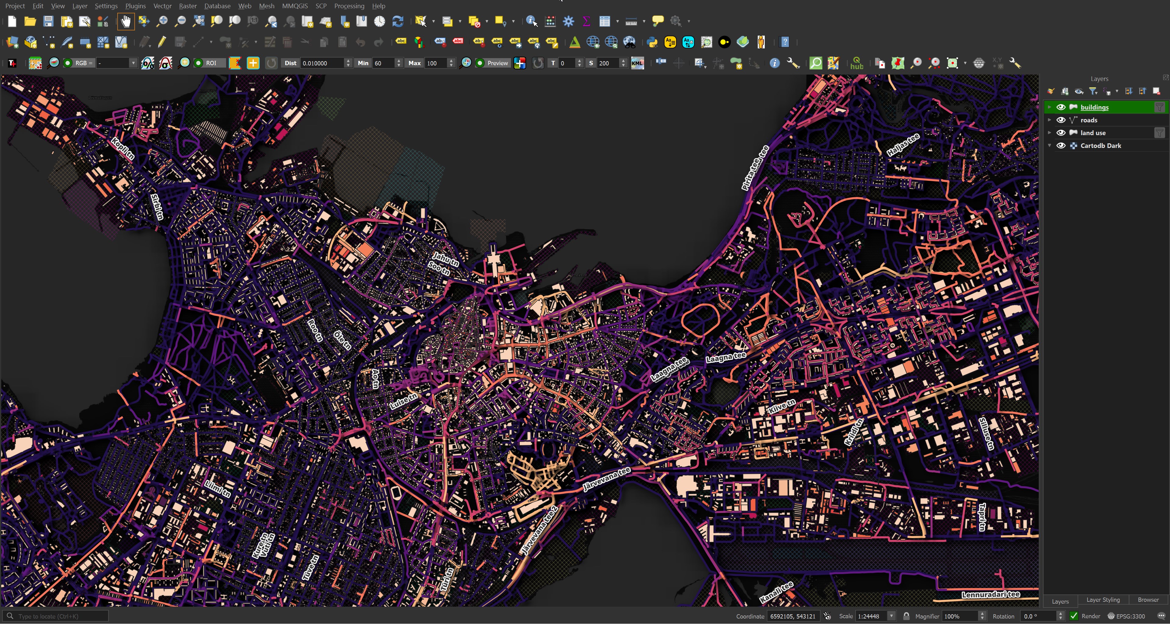
Below is a rendering of the Estonian Land Board's building and road data for Tallinn (the land use data came from OSM via Overture). They've done a good job of segmenting the data into separate files and making sure the metadata for each file is well-populated. This makes it easy to drop the Shapefiles onto QGIS and pick a field to colour-code each feature on. This map took a few minutes to put together with most of that time spent playing with different colour schemes.
I did look around for OSM tools that can extract features from OSM files and place them into themed GeoPackage files but I couldn't find any. So I spent yesterday putting together a script to do just that.
In this post, I'll walk through using my OSM Split script.
Installing Prerequisites
The following was run on Ubuntu for Windows which is based on Ubuntu 20.04 LTS. The system is powered by an Intel Core i5 4670K running at 3.40 GHz and has 32 GB of RAM. The primary partition is a 2 TB Samsung 870 QVO SSD.
My script is written in Python and uses GDAL to convert GeoJSON intermediate files into GeoPackages.
$ sudo apt update
$ sudo apt install \
    gdal-bin \
    python3-pip \
    python3-virtualenv
I'll set up a Python Virtual Environment and install my script's dependencies.
$ virtualenv ~/.osm
$ source ~/.osm/bin/activate

$ git clone https://github.com/marklit/osm_split
$ python -m pip install -r osm_split/requirements.txt
I'll also use DuckDB, along with its JSON and Spatial extensions, in this post to extract data from OSM's PBF files.
$ cd ~
$ wget -c https://github.com/duckdb/duckdb/releases/download/v0.10.0/duckdb_cli-linux-amd64.zip
$ unzip -j duckdb_cli-linux-amd64.zip
$ chmod +x duckdb
$ ~/duckdb
INSTALL json;
INSTALL spatial;
I'll set up DuckDB to load all the extensions each time it launches.
$ vi ~/.duckdbrc
.timer on
.width 180
LOAD json;
LOAD spatial;
The maps in this post were rendered with QGIS version 3.34. QGIS is a desktop application that runs on Windows, macOS and Linux.
I used QGIS' Tile+ plugin to add basemaps onto some of the maps below.
Extracting Features
I'll download the latest version of the Estonian OSM dataset. This PBF is ~100 MB.
$ wget -qO 2023-11-29.osm.pbf \
           https://download.geofabrik.de/europe/estonia-latest.osm.pbf
I'll then run my OSM split script to break up the features into individual GeoPackage files.
$ python3 osm_split/main.py \
          2023-11-28.osm.pbf
The above took ~20 minutes to convert the above PBF file into 1,087 themed GeoPackage files.
Categorising (lines).. ━━━━━━━━━━━━━━━━━━━━━━━━━━━━━━━━━━━━━━━━ 100% 0:12:10
GeoJSON to GPKG (lines).. ━━━━━━━━━━━━━━━━━━━━━━━━━━━━━━━━━━━━━━━━ 100% 0:05:30
Categorising (multilinestrings).. ━━━━━━━━━━━━━━━━━━━━━━━━━━━━━━━━━━━━━━━━ 100% 0:00:23
GeoJSON to GPKG (multilinestrings).. ━━━━━━━━━━━━━━━━━━━━━━━━━━━━━━━━━━━━━━━━ 100% 0:00:13
Categorising (multipolygons).. ━━━━━━━━━━━━━━━━━━━━━━━━━━━━━━━━━━━━━━━━ 100% 0:00:43
GeoJSON to GPKG (multipolygons).. ━━━━━━━━━━━━━━━━━━━━━━━━━━━━━━━━━━━━━━━━ 100% 0:00:51
Categorising (points).. ━━━━━━━━━━━━━━━━━━━━━━━━━━━━━━━━━━━━━━━━ 100% 0:01:45
GeoJSON to GPKG (points).. ━━━━━━━━━━━━━━━━━━━━━━━━━━━━━━━━━━━━━━━━ 100% 0:01:40
Below are the aggregate file sizes and file counts for each geometry type.
        geometry | file count | size (MB)
-----------------|------------|----------
lines            |        416 |      657
multipolygons    |         94 |      119
points           |        563 |       43
multilinestrings |         14 |       32
Themed GeoPackages
In the points dataset, there are 208 shop types. Here are the ten most common types.
$ ls -lhtS points/shop/ | head
... 131K ... clothes.gpkg
...  95K ... convenience.gpkg
...  85K ... supermarket.gpkg
...  72K ... car_repair.gpkg
...  63K ... beauty.gpkg
...  51K ... florist.gpkg
...  51K ... hairdresser.gpkg
...  43K ... furniture.gpkg
...  30K ... gift.gpkg
Most files are a few MB at most but the lines/building.gpkg makes up ~40% of the dataset. Outside of location, there wasn't a lot of metadata to segment this file on. I've run my script on a few medium-sized countries but there could be richer metadata in places I haven't yet explored.
That said, some Estonian building data does contain some useful metadata and those records have been broken up into 110 individual GeoPackage files.
$ ls -lhtS lines/building/ | head -n20
... 5.2M ... house.gpkg
... 4.5M ... apartments.gpkg
... 2.4M ... greenhouse.gpkg
... 1.6M ... garage.gpkg
... 1.2M ... detached.gpkg
... 846K ... garages.gpkg
... 758K ... ruins.gpkg
... 673K ... retail.gpkg
... 587K ... residential.gpkg
... 489K ... industrial.gpkg
... 391K ... construction.gpkg
... 361K ... school.gpkg
... 332K ... service.gpkg
... 294K ... terrace.gpkg
... 286K ... semidetached_house.gpkg
... 256K ... church.gpkg
... 220K ... historic.gpkg
... 203K ... office.gpkg
... 192K ... commercial.gpkg
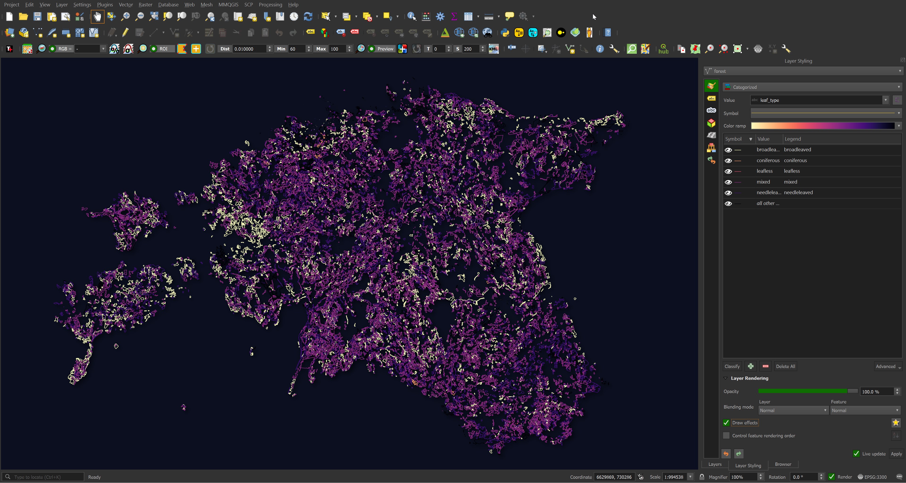
Because the other_tags field was converted into GeoJSON properties, the tags are easy to use for categorisation in QGIS. Below are the forests of Estonia coloured by leaf type.
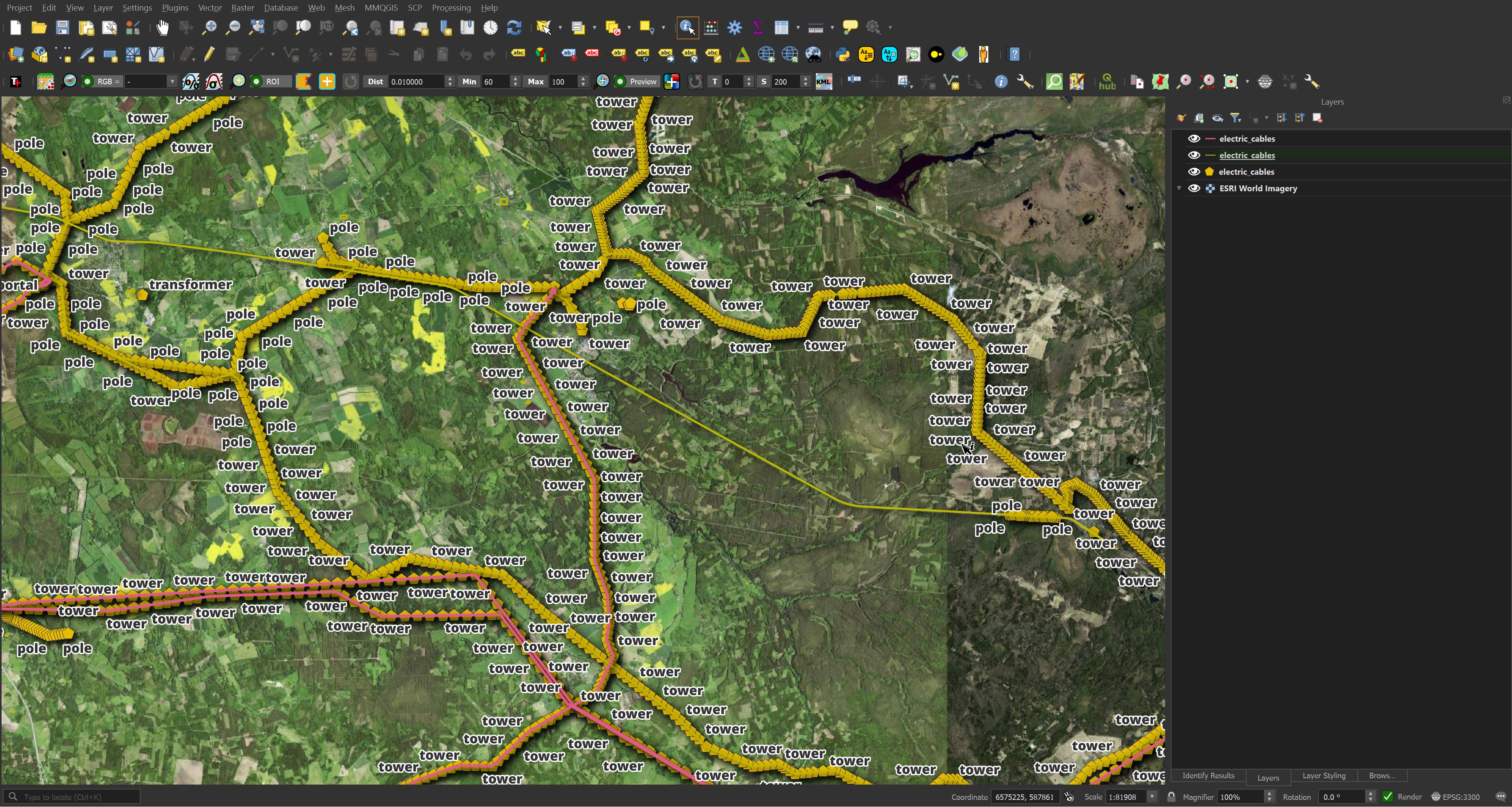
Some types of data can span multiple types of geometry. Below are the three electric cable datasets.
$ ls -lht */electric_cables.gpkg
... 7.3M ... points/electric_cables.gpkg
... 513K ... multilinestrings/electric_cables.gpkg
... 3.6M ... lines/electric_cables.gpkg
Below is a rendering of the above in QGIS. I've labeled the points with the types of infrastructure they represent.
Most of the data in lines/coastline.gpkg was supplied by the Estonian Land Board over the past 15 years.
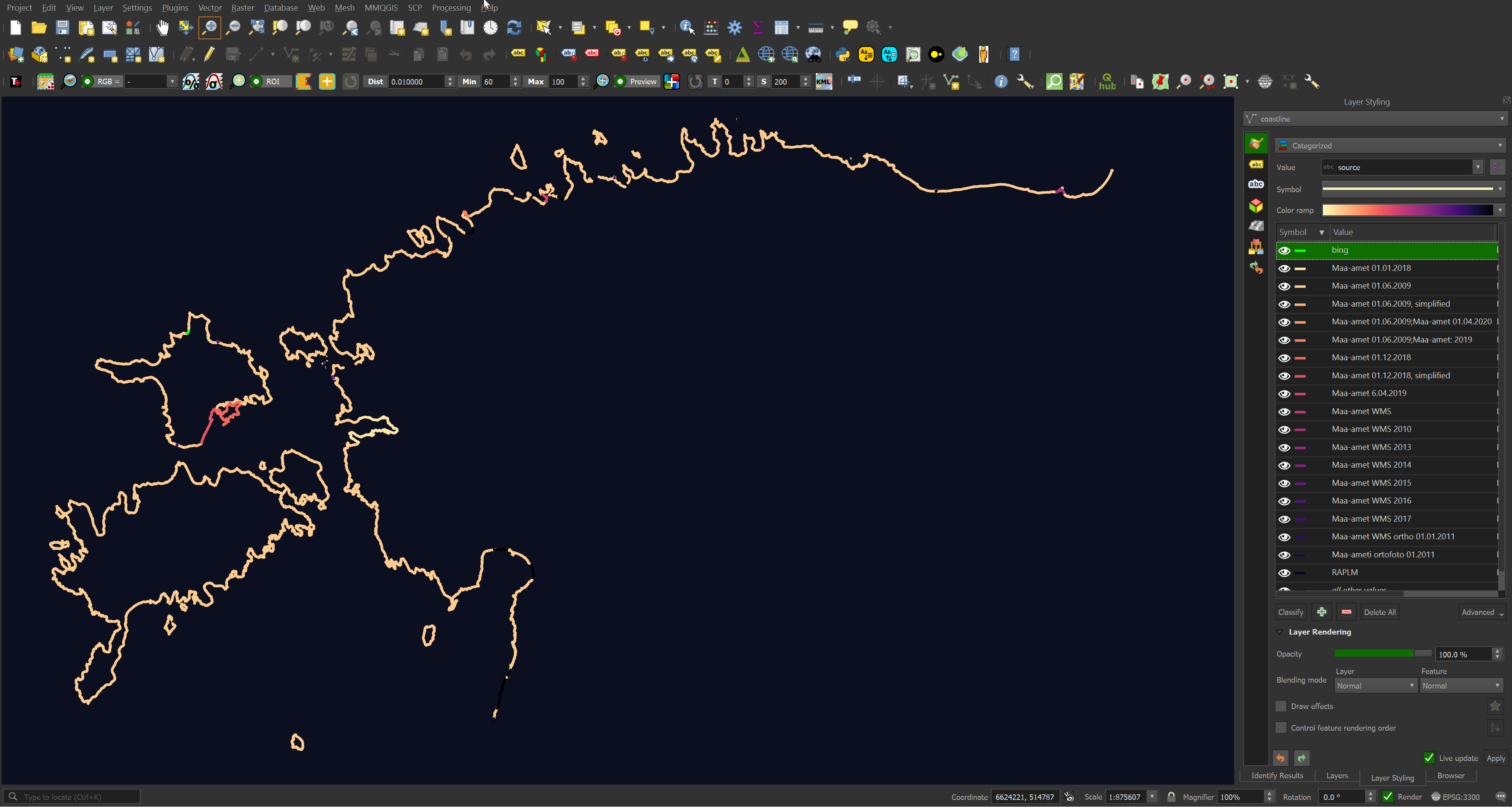
Each attribute from the other_tags field can now be addressed as its own column. Below I'll find the most common voltages for the above power lines.
$ ~/duckdb
SELECT voltage,
       COUNT(*)
FROM ST_READ('lines/electric_cables.gpkg')
WHERE LENGTH(voltage)
GROUP BY 1
ORDER BY 2 DESC
LIMIT 1;
┌──────────────┬──────────────┐
│   voltage    │ count_star() │
│   varchar    │    int64     │
├──────────────┼──────────────┤
│ 10000        │          508 │
│ 110000       │          482 │
│ 35000        │          318 │
│ 3000         │          257 │
│ 400          │          237 │
│ 600          │          134 │
│ 330000       │           99 │
│ 20000        │           84 │
│ 1000         │           78 │
│ 110000;10000 │           45 │
├──────────────┴──────────────┤
│ 10 rows           2 columns │
└─────────────────────────────┘