Natural Earth is a mapping dataset produced by volunteers from around the world and published into the public domain.
The volunteer efforts are led by Tom Patterson, a retired Cartographer from Virginia who worked for the National Park Service and Nathaniel Vaughn Kelso, who has worked in Cartography roles at Apple, Mapzen, National Geographic and the Washington Post.
The project produces ~170 datasets across three major categories. Below I've layered ten of these datasets on top of one another. These include water depths, country boundaries, disputed regions, Antarctic claims, time zones, railroads, airports (rendered as a heatmap), urban areas, shipping ports and maritime indicators.
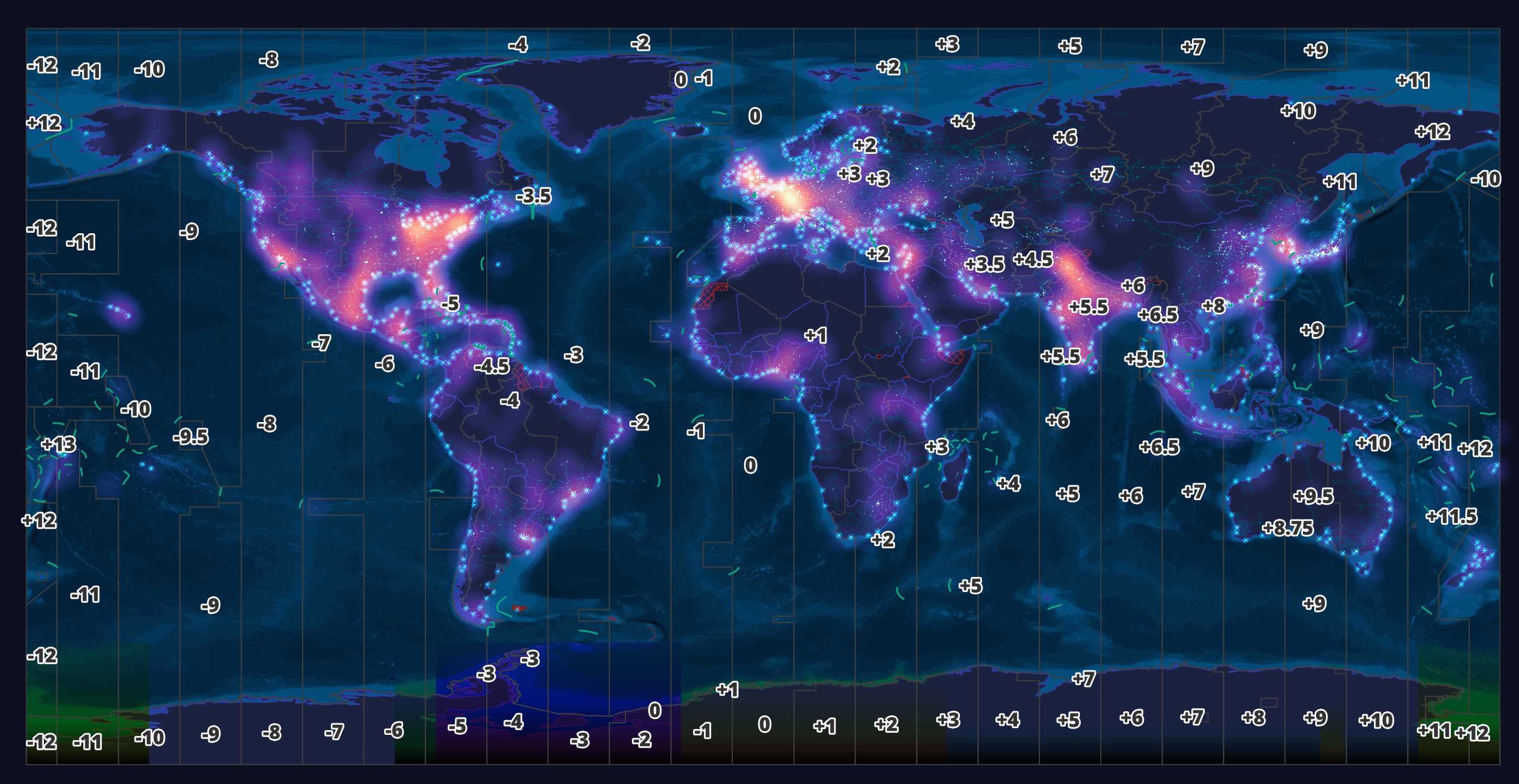
The above rendering was produced solely with vector data with no basemaps or raster data being used.
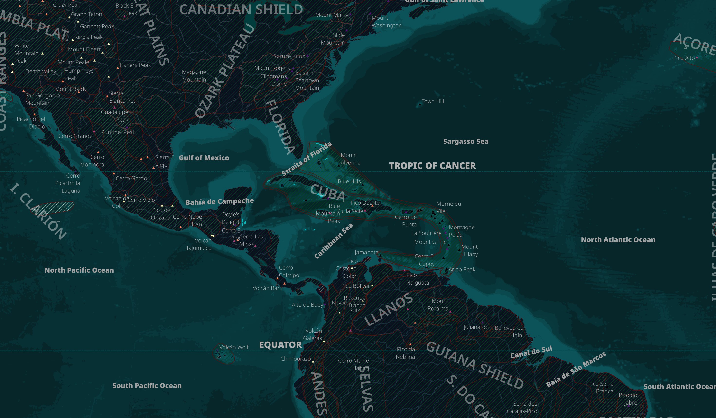
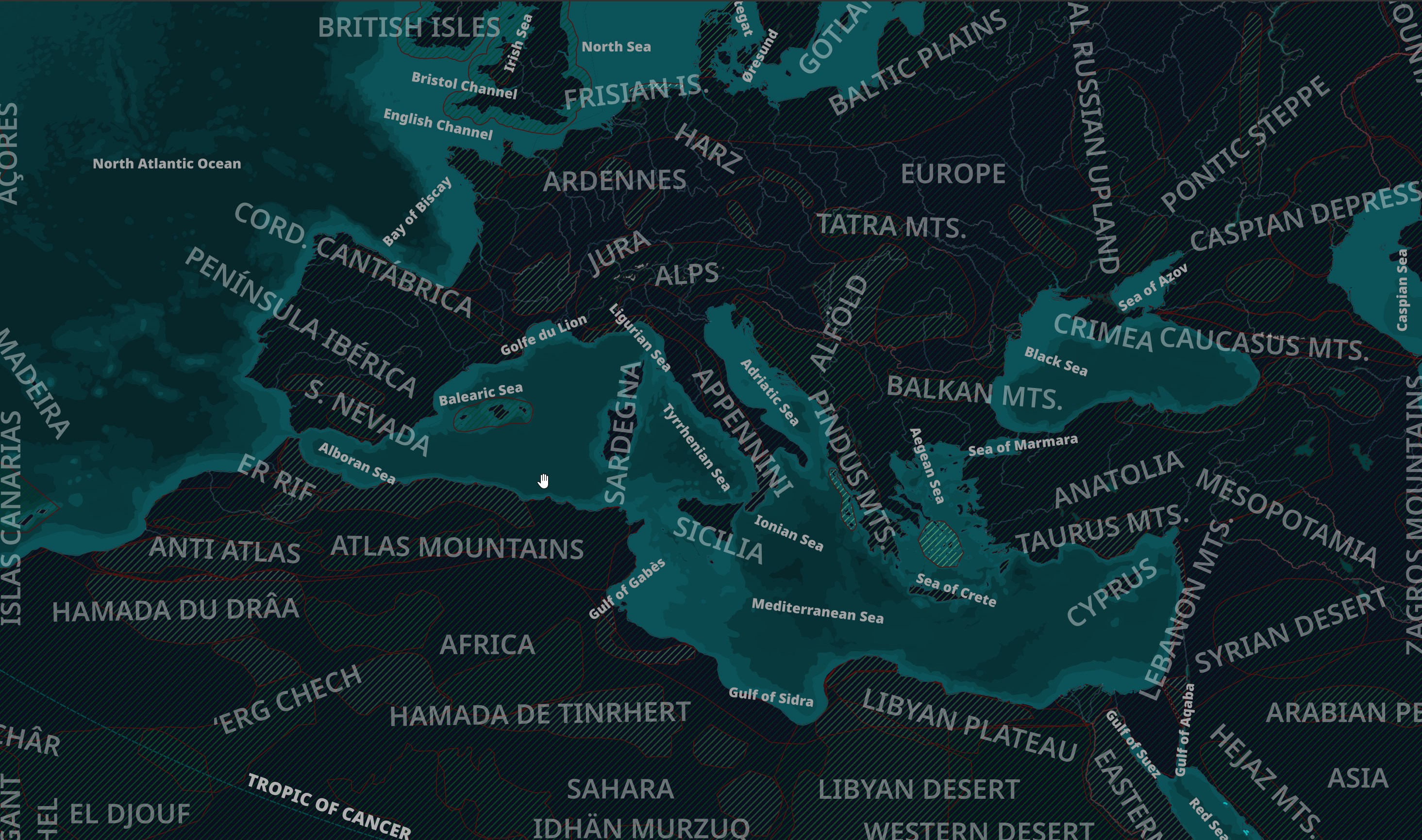
Below I've rendered their regions, coastlines, lakes, reefs, rivers, glaciated areas, marines and elevation points datasets atop their water depth polygons.
In this post, I'll download and examine Natural Earth's freely available global geospatial datasets.
Installing Prerequisites
The following was run on Ubuntu for Windows which is based on Ubuntu 20.04 LTS. The system is powered by an Intel Core i5 4670K running at 3.40 GHz and has 32 GB of RAM. The primary partition is a 2 TB Samsung 870 QVO SSD.
I'll be using AWS S3 to download these datasets.
$ sudo apt update
$ sudo apt install \
    awscli \
    exiftool
I'll use DuckDB, along with its JSON and Spatial extensions, in this post.
$ cd ~
$ wget -c https://github.com/duckdb/duckdb/releases/download/v0.9.1/duckdb_cli-linux-amd64.zip
$ unzip -j duckdb_cli-linux-amd64.zip
$ chmod +x duckdb
$ ~/duckdb
INSTALL json;
INSTALL spatial;
I'll set up DuckDB to load all these extensions each time it launches.
$ vi ~/.duckdbrc
.timer on
.width 180
LOAD json;
LOAD spatial;
The maps in this post were rendered with QGIS version 3.34. QGIS is a desktop application that runs on Windows, macOS and Linux.
I used QGIS' Tile+ plugin to add satellite basemaps when it helps provide visual context around Natural Earth's vector data.
Downloading Natural Earth's Datasets
The datasets are available at 1:10m (most detailed), 1:50m, and 1:110 million scales. I'll download version 5.1.2 of the 1:10m scale dataset for this exercise. It was published in May of last year.
$ mkdir -p ~/naturalearth

$ for DATASET in cultural physical raster; do
      cd ~/naturalearth
      aws s3 sync \
            --no-sign-request \
            s3://naturalearth/10m_$DATASET/ \
            10m_$DATASET/

      cd 10m_$DATASET/
      ls *.zip | xargs -n1 -P4 -I% unzip -qn %
  done
The above downloaded three categories of data. In ZIP format, there is 120 MB of physical data (coastlines, lakes, etc..) across 54 ZIP files, 720 MB of cultural data (transport, time zones, populated areas, borders) across 79 ZIP files and 5.6 GB of raster data (relief maps of the earth) across 37 ZIP files.
Data Shipped as Shapefiles
The physical and cultural datasets contain Shapefiles inside their respective ZIP files. These are a multi-file format and have been one of the primary ways geospatial data has been shared for the past few decades. It was popularised by the now 650K organisations that use Esri software.
Below is the airports dataset.
$ cd ~/naturalearth/10m_cultural
$ unzip -l ne_10m_airports.zip
Archive:  ne_10m_airports.zip
  Length      Date    Time    Name
---------  ---------- -----   ----
    37654  2021-12-08 02:24   ne_10m_airports.README.html
        7  2021-12-08 02:24   ne_10m_airports.VERSION.txt
        5  2021-08-01 20:23   ne_10m_airports.cpg
  6694349  2021-08-29 09:05   ne_10m_airports.dbf
      145  2021-08-29 09:05   ne_10m_airports.prj
    25104  2021-08-01 20:23   ne_10m_airports.shp
     7244  2021-08-01 20:23   ne_10m_airports.shx
---------                     -------
  6764508                     7 files
The PRJ file contains the projection information.
$ cat ne_10m_airports.prj
GEOGCS["GCS_WGS_1984",DATUM["D_WGS_1984",SPHEROID["WGS_1984",6378137.0,298.257223563]],PRIMEM["Greenwich",0.0],UNIT["Degree"
The CPG file contains the character encoding. In this case, it's UTF-8.
$ hexdump -C ne_10m_airports.cpg
00000000  55 54 46 2d 38                                    |UTF-8|
00000005
The DBF file contains a database table and will often hold all non-vector data for each record within the dataset.
This format was originally introduced by dBase in the late 1970s and was popular with Microsoft's FoxPro in the 1990s. NCR Corporation produces point-of-sale (POS) systems found in many restaurants, shops and hotels and still supports writing sales and operations data to DBF files.
The SHP file stores geometry and the SHX file contains indices.
You can use DuckDB's Spatial Extension to work with Shapefiles using SQL. Below is the record for Tallinn Airport. I've excluded any field names prefixed with name_.
$ ~/duckdb
.mode line

SELECT COLUMNS(c -> c NOT LIKE 'name_%')
FROM   ST_READ('ne_10m_airports.shx')
WHERE  abbrev = 'TLL'
LIMIT  1;
 scalerank = 4
featurecla = Airport
      type = major
      name = Ulemiste
    abbrev = TLL
  location = terminal
  gps_code = EETN
 iata_code = TLL
 wikipedia = http://en.wikipedia.org/wiki/Tallinn_Airport
 natlscale = 50.0
  comments =
wikidataid = Q630524
wdid_score = 4
     ne_id = 1159126123
      geom = POINT (24.798964869982985 59.41650146974512)
Unlike CSVs, Shapefiles are strongly typed. They also differentiate between integers and doubles, unlike JSON files. The vector data is stored as a GEOMETRY type so no type casting will be needed prior to any analysis.
DESCRIBE SELECT COLUMNS(c -> c NOT LIKE 'name_%')
FROM ST_READ('ne_10m_airports.shx')
LIMIT 1;
┌─────────────┬─────────────┬─────────┬─────────┬─────────┬─────────┐
│ column_name │ column_type │  null   │   key   │ default │  extra  │
│   varchar   │   varchar   │ varchar │ varchar │ varchar │ varchar │
├─────────────┼─────────────┼─────────┼─────────┼─────────┼─────────┤
│ scalerank   │ INTEGER     │ YES     │         │         │         │
│ featurecla  │ VARCHAR     │ YES     │         │         │         │
│ type        │ VARCHAR     │ YES     │         │         │         │
│ name        │ VARCHAR     │ YES     │         │         │         │
│ abbrev      │ VARCHAR     │ YES     │         │         │         │
│ location    │ VARCHAR     │ YES     │         │         │         │
│ gps_code    │ VARCHAR     │ YES     │         │         │         │
│ iata_code   │ VARCHAR     │ YES     │         │         │         │
│ wikipedia   │ VARCHAR     │ YES     │         │         │         │
│ natlscale   │ DOUBLE      │ YES     │         │         │         │
│ comments    │ VARCHAR     │ YES     │         │         │         │
│ wikidataid  │ VARCHAR     │ YES     │         │         │         │
│ wdid_score  │ INTEGER     │ YES     │         │         │         │
│ ne_id       │ BIGINT      │ YES     │         │         │         │
│ geom        │ GEOMETRY    │ YES     │         │         │         │
├─────────────┴─────────────┴─────────┴─────────┴─────────┴─────────┤
│ 15 rows                                                 6 columns │
└───────────────────────────────────────────────────────────────────┘
Misplaced Borders
There are a large number of fields listing facts and alternative names for 258 countries and territories around the world in Natural Earth's Administrative dataset.
$ cd ~/naturalearth
$ ~/duckdb
.mode line

SELECT COLUMNS(c -> c NOT LIKE 'NAME_%' AND
                    c NOT LIKE 'FCLASS_%' AND
                    c NOT LIKE '%_A3%' AND
                    c != 'geom')
FROM ST_READ('10m_cultural/ne_10m_admin_0_countries.shx')
WHERE ISO_A2 = 'EE'
LIMIT 1;
featurecla = Admin-0 country
 scalerank = 0
 LABELRANK = 6
SOVEREIGNT = Estonia
  ADM0_DIF = 0
     LEVEL = 2
      TYPE = Sovereign country
       TLC = 1
     ADMIN = Estonia
  GEOU_DIF = 0
   GEOUNIT = Estonia
    SU_DIF = 0
   SUBUNIT = Estonia
  BRK_DIFF = 0
      NAME = Estonia
  BRK_NAME = Estonia
 BRK_GROUP =
    ABBREV = Est.
    POSTAL = EST
 FORMAL_EN = Republic of Estonia
 FORMAL_FR =
 NOTE_ADM0 =
  NOTE_BRK =
 MAPCOLOR7 = 3
 MAPCOLOR8 = 2
 MAPCOLOR9 = 1
MAPCOLOR13 = 10
   POP_EST = 1326590.0
  POP_RANK = 12
  POP_YEAR = 2019
    GDP_MD = 31471
  GDP_YEAR = 2019
   ECONOMY = 2. Developed region: nonG7
INCOME_GRP = 1. High income: OECD
   FIPS_10 = EN
    ISO_A2 = EE
 ISO_A2_EH = EE
    ISO_N3 = 233
 ISO_N3_EH = 233
     WB_A2 = EE
    WOE_ID = 23424805
 WOE_ID_EH = 23424805
  WOE_NOTE = Exact WOE match as country
  ADM0_ISO = EST
 ADM0_DIFF =
  ADM0_TLC = EST
 CONTINENT = Europe
 REGION_UN = Europe
 SUBREGION = Northern Europe
 REGION_WB = Europe & Central Asia
  LONG_LEN = 7
ABBREV_LEN = 4
      TINY = -99
  HOMEPART = 1
  MIN_ZOOM = 0.0
 MIN_LABEL = 3.0
 MAX_LABEL = 8.0
   LABEL_X = 25.867126
   LABEL_Y = 58.724865
     NE_ID = 1159320615
WIKIDATAID = Q191
  TLC_DIFF =
This is the country count broken down by continent.
SELECT   COUNT(*),
         CONTINENT
FROM     ST_READ('10m_cultural/ne_10m_admin_0_countries.shx')
WHERE    featurecla = 'Admin-0 country'
GROUP BY 2
ORDER BY 2;
┌──────────────┬─────────────────────────┐
│ count_star() │        CONTINENT        │
│    int64     │         varchar         │
├──────────────┼─────────────────────────┤
│           55 │ Africa                  │
│            1 │ Antarctica              │
│           59 │ Asia                    │
│           51 │ Europe                  │
│           42 │ North America           │
│           26 │ Oceania                 │
│            9 │ Seven seas (open ocean) │
│           15 │ South America           │
└──────────────┴─────────────────────────┘
The geometry for the borders themselves is pretty far off what you'd find with OpenStreetMap (OSM). The red line is the border taken from OSM and the yellow line is the border found in Natural Earth's latest release.
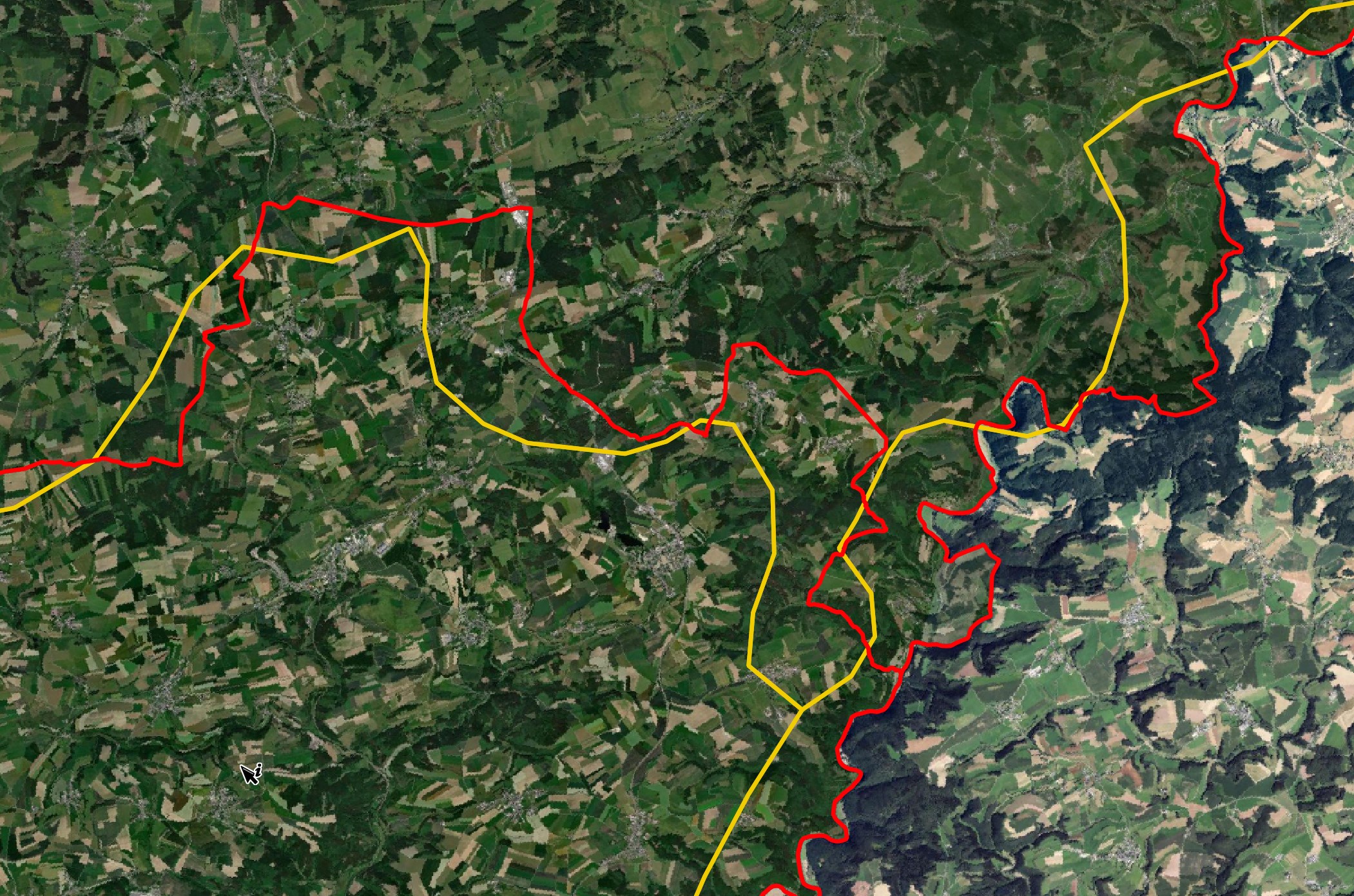
I found similar misplacements with just about every country in Europe. I raised a ticket with the project so hopefully this gets addressed in the next release.
There are nine islands not attributed to any one continent but instead are classed as being on the open ocean.
SELECT   SOVEREIGNT,
         NAME_LONG,
         ECONOMY,
         INCOME_GRP
FROM     ST_READ('10m_cultural/ne_10m_admin_0_countries.shx')
WHERE    CONTINENT = 'Seven seas (open ocean)'
ORDER BY 1, 2;
┌────────────────┬─────────────────────────────────────┬────────────────────────────┬─────────────────────────┐
│   SOVEREIGNT   │              NAME_LONG              │          ECONOMY           │       INCOME_GRP        │
│    varchar     │               varchar               │          varchar           │         varchar         │
├────────────────┼─────────────────────────────────────┼────────────────────────────┼─────────────────────────┤
│ Australia      │ Heard I. and McDonald Islands       │ 7. Least developed region  │ 5. Low income           │
│ France         │ Clipperton Island                   │ 7. Least developed region  │ 5. Low income           │
│ France         │ French Southern and Antarctic Lands │ 6. Developing region       │ 2. High income: nonOECD │
│ Maldives       │ Maldives                            │ 6. Developing region       │ 3. Upper middle income  │
│ Mauritius      │ Mauritius                           │ 6. Developing region       │ 3. Upper middle income  │
│ Seychelles     │ Seychelles                          │ 6. Developing region       │ 3. Upper middle income  │
│ United Kingdom │ British Indian Ocean Territory      │ 2. Developed region: nonG7 │ 2. High income: nonOECD │
│ United Kingdom │ Saint Helena                        │ 6. Developing region       │ 4. Lower middle income  │
│ United Kingdom │ South Georgia and the Islands       │ 7. Least developed region  │ 5. Low income           │
└────────────────┴─────────────────────────────────────┴────────────────────────────┴─────────────────────────┘
The disputed territories table has a lot of detail within it. This is a summary of its records.
SELECT   FEATURECLA,
         FCLASS_OSM,
         COUNT(*)
FROM     ST_READ('10m_cultural/ne_10m_admin_0_boundary_lines_disputed_areas.shx')
GROUP BY 1, 2
ORDER BY 1, 2;
┌──────────────────┬─────────────────────────────────┬──────────────┐
│    FEATURECLA    │           FCLASS_OSM            │ count_star() │
│     varchar      │             varchar             │    int64     │
├──────────────────┼─────────────────────────────────┼──────────────┤
│ Breakaway        │ Admin-1 boundary                │            2 │
│ Breakaway        │ Unrecognized                    │           16 │
│ Claim boundary   │ International boundary (verify) │            9 │
│ Claim boundary   │ Unrecognized                    │           32 │
│ Elusive frontier │ Unrecognized                    │            2 │
│ Reference line   │ Unrecognized                    │           14 │
└──────────────────┴─────────────────────────────────┴──────────────┘
Regions and Lakes
There are 1,355 Lakes in the dataset. 116 are listed as having a dam. Below is a dam count by country.
CREATE OR REPLACE TABLE countries AS
    SELECT Name,
           CONTINENT,
           geom
    FROM   ST_READ('10m_cultural/ne_10m_admin_0_countries.shx')
    WHERE  featurecla = 'Admin-0 country';

SELECT   b.CONTINENT continent,
         b.Name country,
         COUNT(*) dam_count
FROM     ST_READ('10m_physical/ne_10m_lakes.shx') a
LEFT JOIN countries b
    ON ST_INTERSECTS(ST_CENTROID(a.geom), b.geom)
WHERE    a.dam_name IS NOT NULL
GROUP BY 1, 2
ORDER BY 1,
         3 DESC;
┌───────────────┬──────────────────────────┬───────────┐
│   continent   │         country          │ dam_count │
│    varchar    │         varchar          │   int64   │
├───────────────┼──────────────────────────┼───────────┤
│ Africa        │ South Africa             │         2 │
│ Africa        │ Zimbabwe                 │         1 │
│ Africa        │ Sudan                    │         1 │
│ Africa        │ Cameroon                 │         1 │
│ Asia          │ India                    │         5 │
│ Asia          │ Thailand                 │         3 │
│ Asia          │ Turkey                   │         3 │
│ Asia          │ Kazakhstan               │         1 │
│ Asia          │ Iraq                     │         1 │
│ Asia          │ Syria                    │         1 │
│ Asia          │ Bangladesh               │         1 │
│ Asia          │ Sri Lanka                │         1 │
│ Asia          │ North Korea              │         1 │
│ Asia          │ Laos                     │         1 │
│ Asia          │ China                    │         1 │
│ Asia          │ Azerbaijan               │         1 │
│ Europe        │ Russia                   │        15 │
│ Europe        │ Finland                  │         6 │
│ Europe        │ Sweden                   │         2 │
│ Europe        │ Ukraine                  │         2 │
│ Europe        │ Spain                    │         1 │
│ North America │ Canada                   │        20 │
│ North America │ United States of America │        20 │
│ North America │ Mexico                   │         5 │
│ North America │ Panama                   │         1 │
│ Oceania       │ Australia                │         3 │
│ Oceania       │ New Zealand              │         2 │
│ South America │ Brazil                   │        12 │
│ South America │ Paraguay                 │         1 │
│ South America │ Venezuela                │         1 │
├───────────────┴──────────────────────────┴───────────┤
│ 30 rows                                    3 columns │
└──────────────────────────────────────────────────────┘
There are 1,047 regions that can overlap with one another. This is the breakdown by continent.
SELECT   REGION,
         COUNT(*)
FROM     ST_READ('10m_physical/ne_10m_geography_regions_polys.shx')
GROUP BY 1
ORDER BY 1;
┌─────────────────────────┬──────────────┐
│         REGION          │ count_star() │
│         varchar         │    int64     │
├─────────────────────────┼──────────────┤
│ Africa                  │          127 │
│ Antarctica              │           97 │
│ Asia                    │          263 │
│ Europe                  │          103 │
│ North America           │          160 │
│ Oceania                 │          200 │
│ Seven seas (open ocean) │           34 │
│ South America           │           63 │
└─────────────────────────┴──────────────┘
This shows the regions in capital letters across Europe, North Africa and Western Asia.
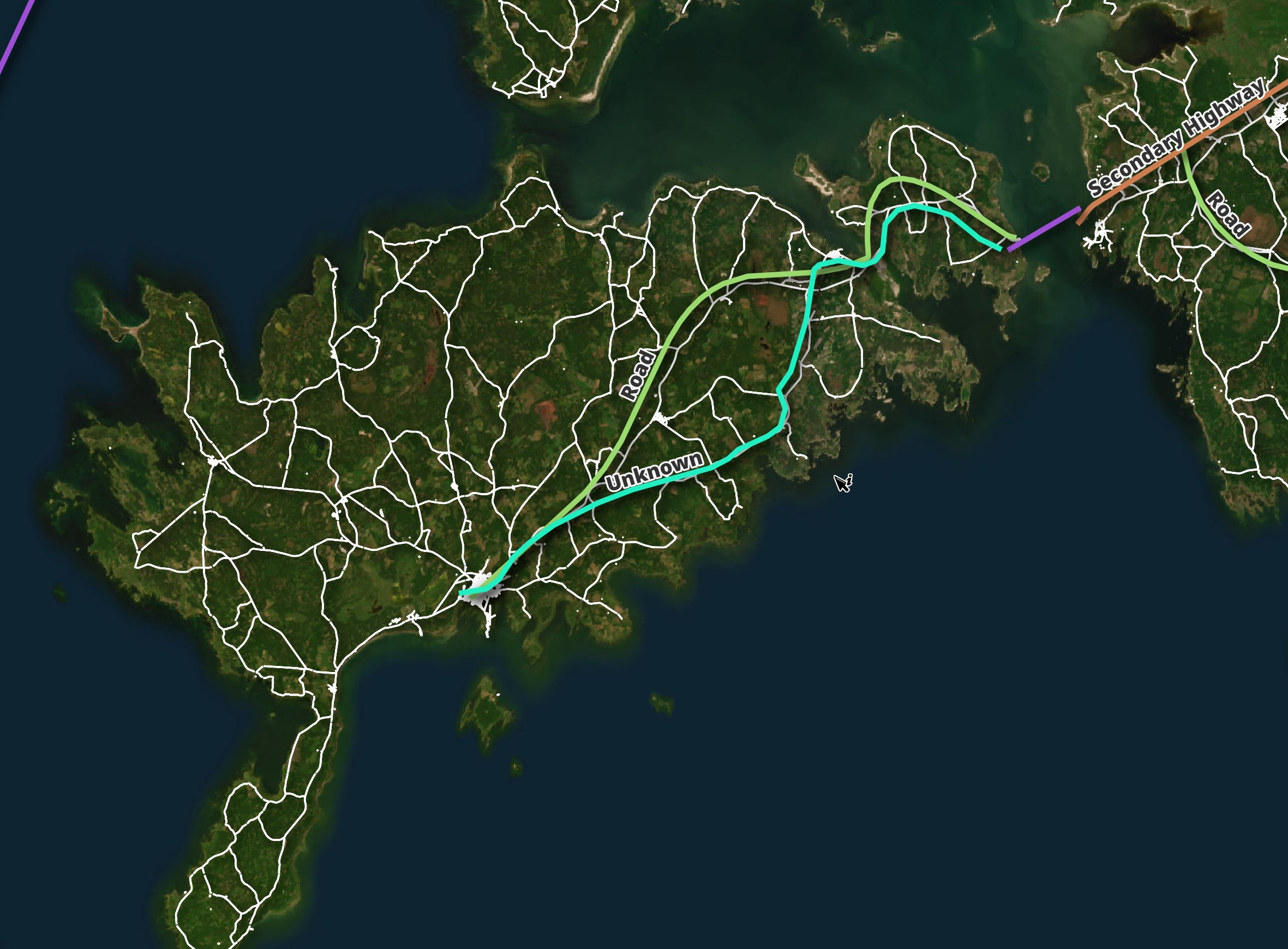
Road Networks
Roads don't change that often but the data here is from two years ago. It'll have a hard time standing up to OSM's daily refreshes. To add to that, the dataset only includes a handful of major roads and they terminate prematurely in some cases.

Below I've left Natural Earth's roads colour-coded and added the Estonian Land Board's road network in white. Even the alignment to the roads' actual geography is off by a fair amount.
Airport Locations
Airports have a decent amount of metadata and look to be fairly complete. I couldn't think of an Airport that wasn't listed in their dataset. Here is a breakdown by type and continent.
SELECT   a."type",
         COUNT(*) FILTER (WHERE b.CONTINENT = 'Africa') AS Africa,
         COUNT(*) FILTER (WHERE b.CONTINENT = 'Asia') AS Asia,
         COUNT(*) FILTER (WHERE b.CONTINENT = 'Europe') AS Europe,
         COUNT(*) FILTER (WHERE b.CONTINENT = 'North America') AS North_America,
         COUNT(*) FILTER (WHERE b.CONTINENT = 'Oceania') AS Oceania,
         COUNT(*) FILTER (WHERE b.CONTINENT = 'South America') AS South_America,
FROM     ST_READ('10m_cultural/ne_10m_airports.shx') a
LEFT JOIN countries b
    ON ST_INTERSECTS(ST_CENTROID(a.geom), b.geom)
GROUP BY 1
ORDER BY North_America DESC;
┌────────────────────┬────────┬───────┬────────┬───────────────┬─────────┬───────────────┐
│        type        │ Africa │ Asia  │ Europe │ North_America │ Oceania │ South_America │
│      varchar       │ int64  │ int64 │ int64  │     int64     │  int64  │     int64     │
├────────────────────┼────────┼───────┼────────┼───────────────┼─────────┼───────────────┤
│ mid                │     82 │    88 │     52 │           131 │      33 │            63 │
│ major              │     14 │   103 │    100 │           118 │      10 │            12 │
│ major and military │      0 │     9 │      1 │             2 │       2 │             0 │
│ mid and military   │      1 │     6 │      4 │             1 │       0 │             2 │
│ spaceport          │      0 │     1 │      1 │             1 │       0 │             0 │
│ military major     │      1 │     1 │      1 │             1 │       0 │             0 │
│ military mid       │      0 │     7 │      2 │             0 │       0 │             0 │
│ military           │      0 │     2 │      0 │             0 │       0 │             0 │
│ small              │      0 │     2 │      0 │             0 │       0 │             0 │
└────────────────────┴────────┴───────┴────────┴───────────────┴─────────┴───────────────┘
There is a 'location' attribute to each airport as well.
SELECT   a.location,
         COUNT(*) FILTER (WHERE b.CONTINENT = 'Africa')        AS Africa,
         COUNT(*) FILTER (WHERE b.CONTINENT = 'Asia')          AS Asia,
         COUNT(*) FILTER (WHERE b.CONTINENT = 'Europe')        AS Europe,
         COUNT(*) FILTER (WHERE b.CONTINENT = 'North America') AS North_America,
         COUNT(*) FILTER (WHERE b.CONTINENT = 'Oceania')       AS Oceania,
         COUNT(*) FILTER (WHERE b.CONTINENT = 'South America') AS South_America,
FROM     ST_READ('10m_cultural/ne_10m_airports.shx') a
LEFT JOIN countries b
    ON ST_INTERSECTS(ST_CENTROID(a.geom), b.geom)
GROUP BY 1
ORDER BY North_America DESC;
┌─────────────┬────────┬───────┬────────┬───────────────┬─────────┬───────────────┐
│  location   │ Africa │ Asia  │ Europe │ North_America │ Oceania │ South_America │
│   varchar   │ int64  │ int64 │ int64  │     int64     │  int64  │     int64     │
├─────────────┼────────┼───────┼────────┼───────────────┼─────────┼───────────────┤
│ terminal    │     90 │   185 │    135 │           229 │      40 │            72 │
│ ramp        │      5 │    18 │     13 │            11 │       2 │             2 │
│ approximate │      0 │     1 │      1 │             5 │       1 │             0 │
│ runway      │      3 │    14 │      9 │             5 │       2 │             3 │
│ parking     │      0 │     1 │      2 │             4 │       0 │             0 │
│ freight     │      0 │     0 │      1 │             0 │       0 │             0 │
└─────────────┴────────┴───────┴────────┴───────────────┴─────────┴───────────────┘
I did a spot check of locations across the globe and I couldn't find a misplaced airport location.
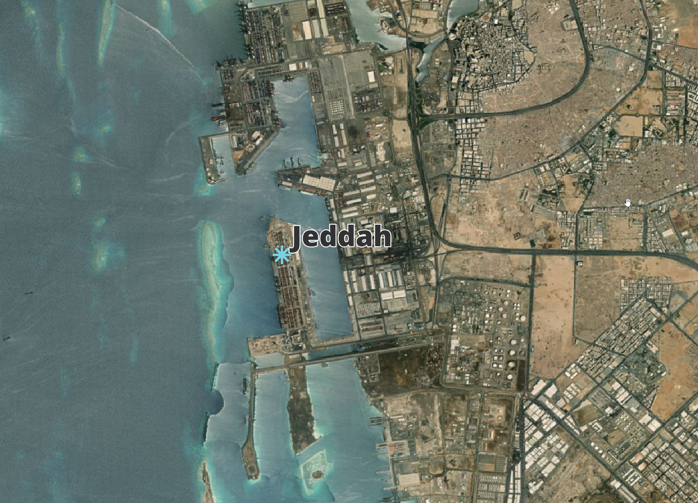
Maritime Ports
There are 1,000 maritime ports. These are the largest ports in Europe, North Africa and the Middle East.
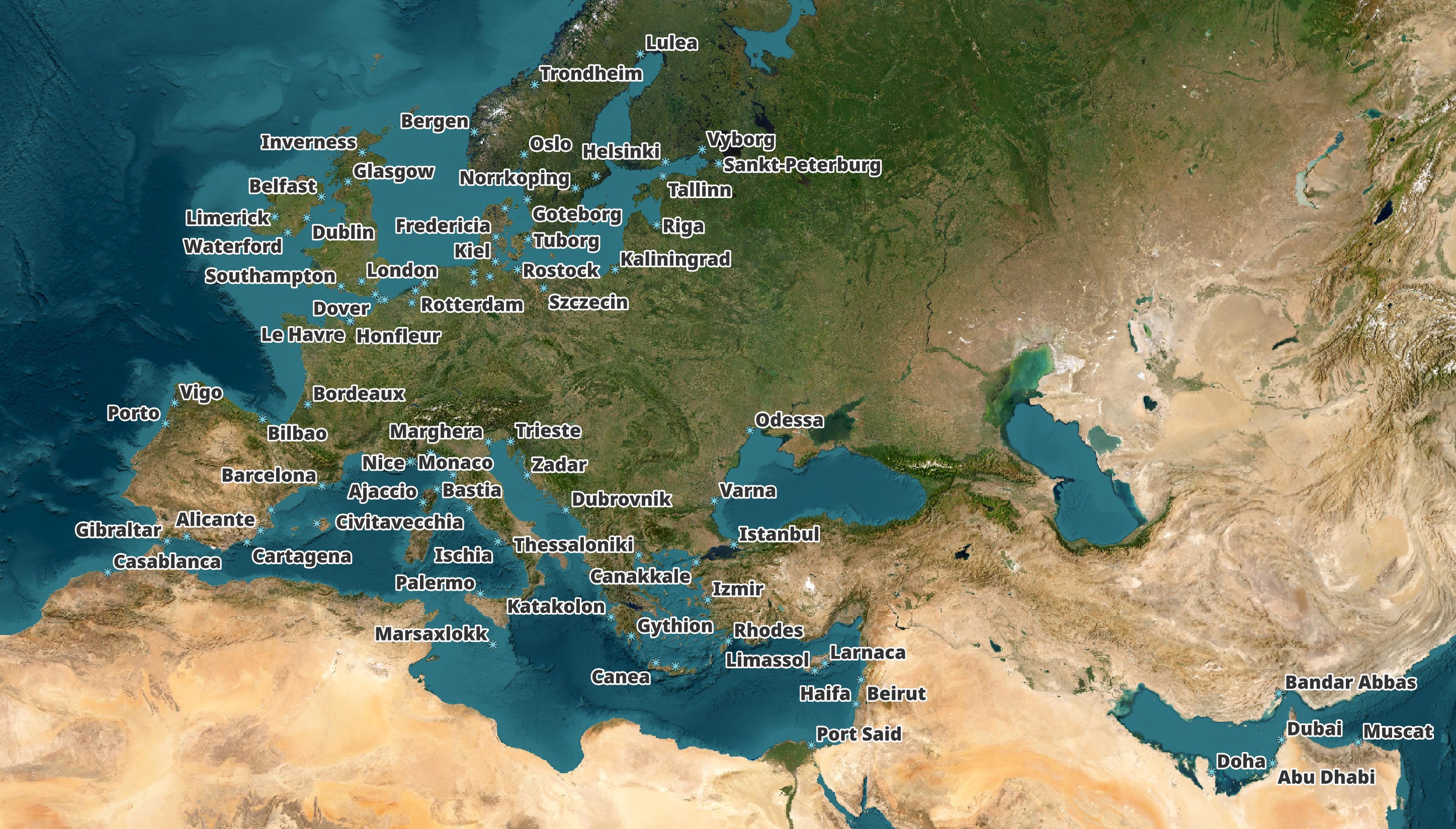
I spot-checked a number of ports and, with the exception of most of the ports in China, most are precisely placed.
Rail Networks
This is the rail network geometry for the entire globe.
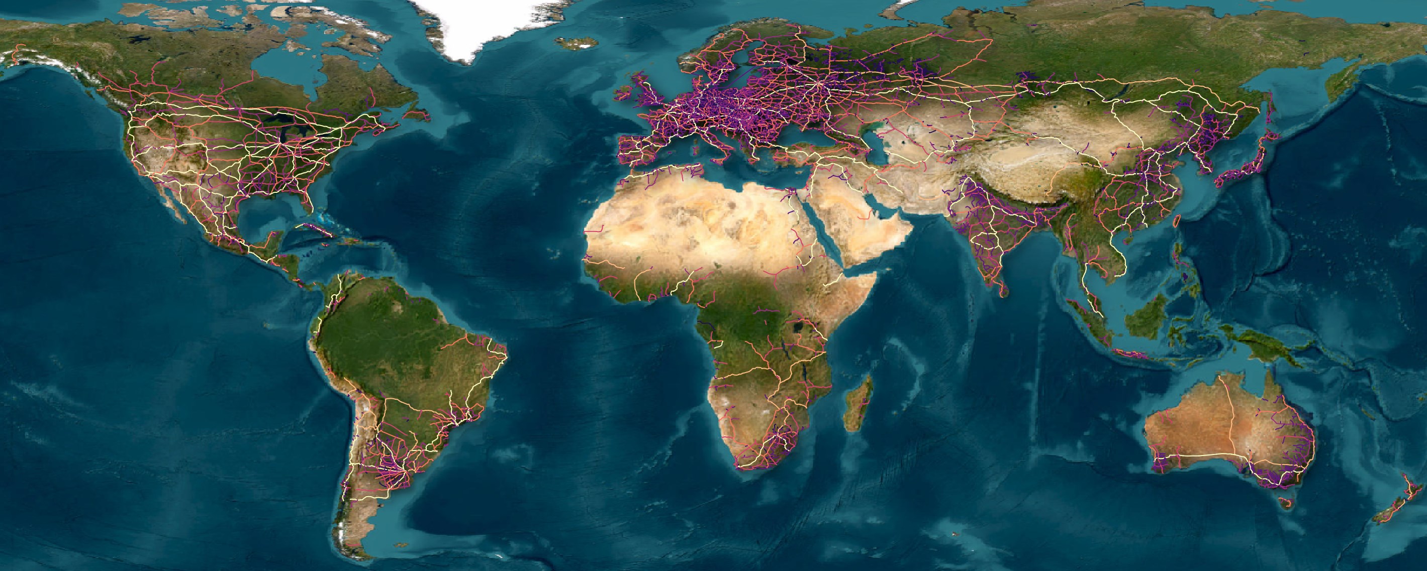
Below are the rail networks across Europe.
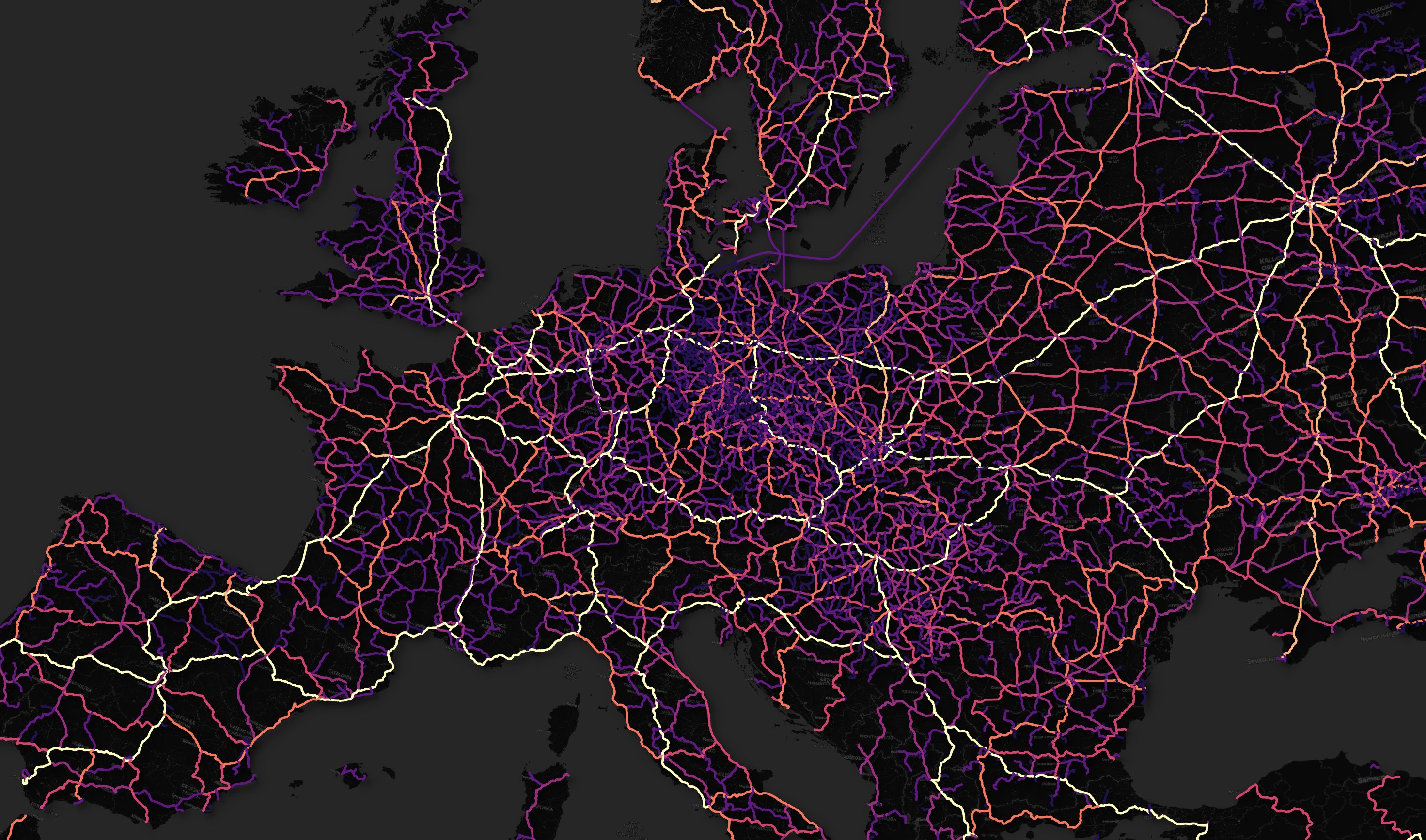
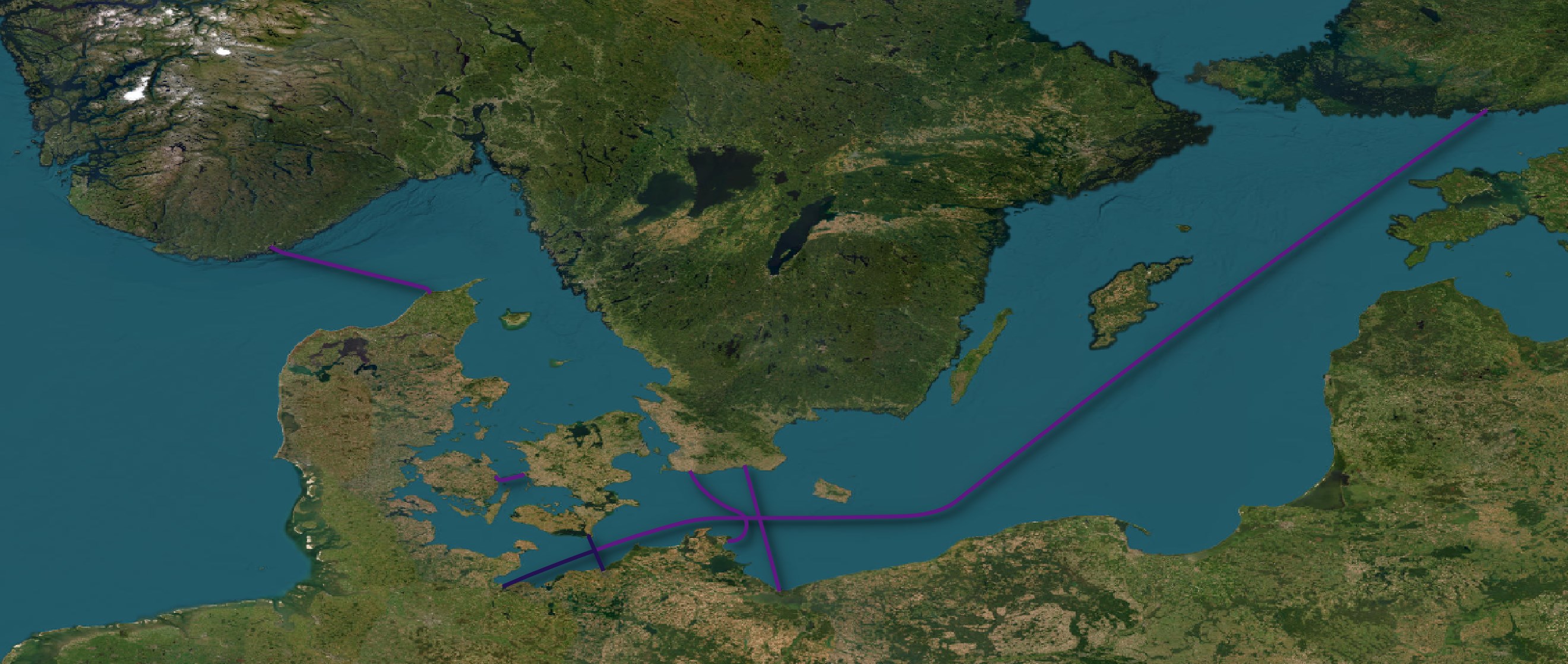
There are also 17 ferry rail lines listed. One is in New Zealand, three are in Japan and the rest are in Europe.
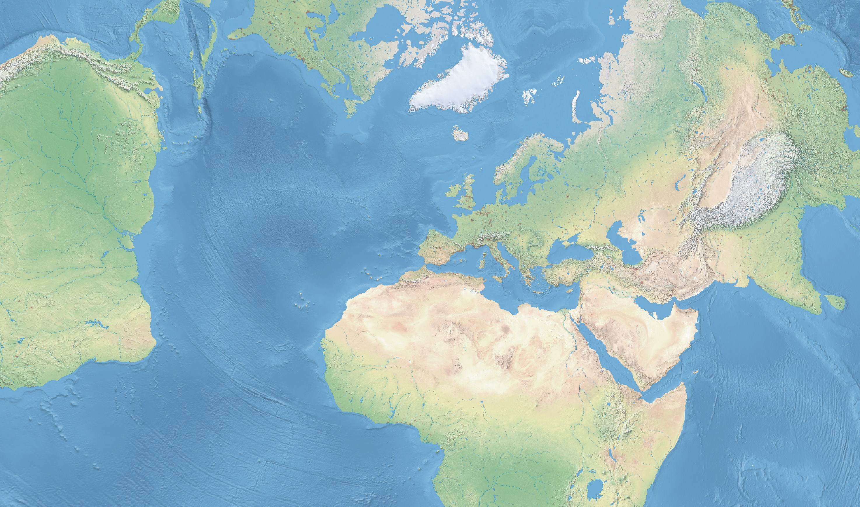
Relief Maps
There are 18 relief / height maps included in the raster dataset. Below is the "Natural Earth II with Shaded Relief, Water, and Drainages" map with the Urban Areas polygons overlay it. The Map is projected in EPSG:3300.
Every TIFF has counterpart files containing projection information. This allows you to drop the TIFF file onto QGIS or ArcGIS Pro and it'll position itself on the globe properly.
They mix and match features and all but the Ocean Bottom map comes in two resolutions. The low-resolution versions are 16200 x 8100 and are denoted by LR in the filename. These are typically around ~320 MB in size. The high-resolution images are 21600 x 10800, contain HR in the filename and are typically ~560 MB in size.
Below I've put together a table in DuckDB with the relief maps details. I'll use this to pull a list of the descriptions of the high-resolution maps.
$ cd ~/naturalearth/10m_raster

$ echo "basename;width;height;bytes;description" > descriptions.csv

$ for FILENAME in *.tif; do
      BASENAME=`echo $FILENAME | sed 's/\.tif//g'`
      WIDTH=`exiftool $FILENAME | grep '^Image Width' | cut -d\: -f2`
      HEIGHT=`exiftool $FILENAME | grep '^Image Height' | cut -d\: -f2`
      DESCRIPTION=`grep '<title>' $BASENAME.README.html | sed 's/<title>//g' | sed 's/ | Natural Earth<\/title>//g'`
      BYTES=`wc -c $FILENAME | cut -d' ' -f1`
      echo "$BASENAME;$WIDTH;$HEIGHT;$BYTES;$DESCRIPTION" >> descriptions.csv
  done

$ ~/duckdb
CREATE OR REPLACE TABLE naturalearth AS
    SELECT *
    FROM READ_CSV('descriptions.csv',
                  delim=';',
                  auto_detect=true)
    ORDER BY width,
             description;

SELECT   basename,
         description
FROM     naturalearth
WHERE    basename LIKE '%HR%'
ORDER BY 2;
┌───────────────────┬─────────────────────────────────────────────────────────────────────────┐
│     basename      │                               description                               │
│      varchar      │                                 varchar                                 │
├───────────────────┼─────────────────────────────────────────────────────────────────────────┤
│ HYP_HR_SR_OB_DR   │ Cross Blended Hypso with Relief, Water, Drains, and Ocean Bottom        │
│ HYP_HR_SR         │ Cross Blended Hypso with Shaded Relief                                  │
│ HYP_HR_SR_W       │ Cross Blended Hypso with Shaded Relief and Water                        │
│ HYP_HR_SR_W_DR    │ Cross Blended Hypso with Shaded Relief, Water, and Drainages            │
│ GRAY_HR_SR        │ Gray Earth with Shaded Relief and Hypsography                           │
│ GRAY_HR_SR_OB_DR  │ Gray Earth with Shaded Relief, Hypsography, Ocean Bottom, and Drainages │
│ GRAY_HR_SR_W      │ Gray Earth with Shaded Relief, Hypsography, and Flat Water              │
│ GRAY_HR_SR_OB     │ Gray Earth with Shaded Relief, Hypsography, and Ocean Bottom            │
│ NE1_HR_LC         │ Natural Earth I                                                         │
│ NE1_HR_LC_SR      │ Natural Earth I with Shaded Relief                                      │
│ NE1_HR_LC_SR_W    │ Natural Earth I with Shaded Relief and Water                            │
│ NE1_HR_LC_SR_W_DR │ Natural Earth I with Shaded Relief, Water, and Drainages                │
│ NE2_HR_LC         │ Natural Earth II                                                        │
│ NE2_HR_LC_SR      │ Natural Earth II with Shaded Relief                                     │
│ NE2_HR_LC_SR_W    │ Natural Earth II with Shaded Relief and Water                           │
│ NE2_HR_LC_SR_W_DR │ Natural Earth II with Shaded Relief, Water, and Drainages               │
│ SR_HR             │ Shaded Relief Basic                                                     │
├───────────────────┴─────────────────────────────────────────────────────────────────────────┤
│ 17 rows                                                                           2 columns │
└─────────────────────────────────────────────────────────────────────────────────────────────┘
Every image includes a documentation file as well.
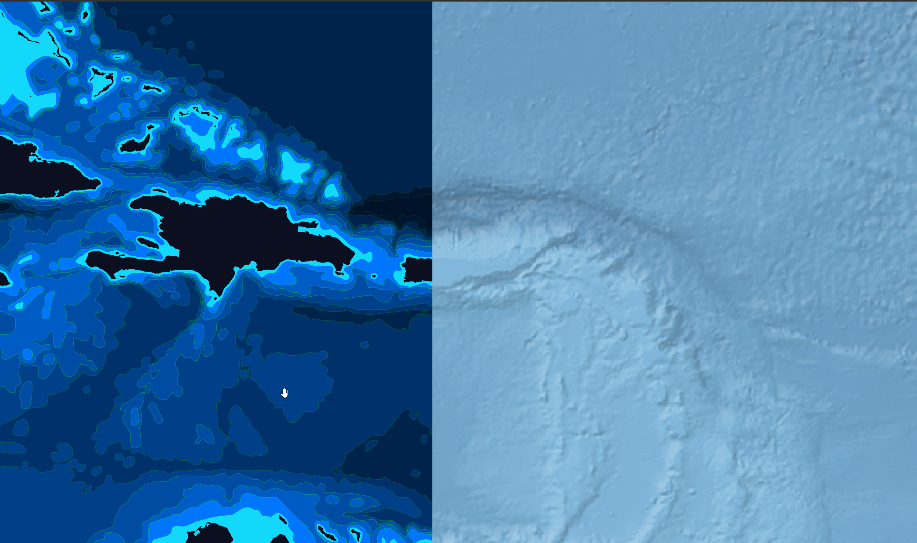
The Ocean Bottom TIFF (OB_LR.tif) looks more detailed than the bathymetry / ocean depth vectors in the physical dataset but it doesn't look as sharp when zoomed into.
That said, this is a single image that can be dropped into a project and might suit your tastes more.
Below I've taken a screenshot of the Caribbean comparing the two. The polygons are on the left and the TIFF is on the right.