A Boeing 787-9 Dreamliner flying nonstop from Newark Liberty International Airport (EWR) to Leonardo da Vinci-Fiumicino Airport (FCO) could need $68K in jet fuel over the 8.5-hour flight. Adjusting the flight path for wind conditions could reduce fuel consumption and possibly save a few thousand dollars.
Firms like Jeppesen have offerings in this space, but Scikit-decide, together with a narrow- and wide-body fuel consumption model built by a professor at the Delft University of Technology and wind data from NOAA, offer an open source solution.
Scikit-decide has been in development for six years. It's a framework for reinforcement learning, automated planning and scheduling. The project can optimise flight paths, re-organise airline workforce schedules and calculate drone swarm paths.
OpenAP is an aircraft performance model and toolkit developed by Dr. Junzi Sun. Dr. Sun has a PhD in air traffic management and, among many other things, teaches a course on the subject as a tenured assistant professor at TU Delft in the Netherlands.
Scikit-decide's optimal flight path solver can be configured to use different fuel consumption models. In this post, I'll compare two flight paths flown using the Airbus A320 and OpenAP's fuel consumption model.
My Workstation
I'm using a 5.7 GHz AMD Ryzen 9 9950X CPU. It has 16 cores and 32 threads and 1.2 MB of L1, 16 MB of L2 and 64 MB of L3 cache. It has a liquid cooler attached and is housed in a spacious, full-sized Cooler Master HAF 700 computer case.
The system has 96 GB of DDR5 RAM clocked at 4,800 MT/s and a 5th-generation, Crucial T700 4 TB NVMe M.2 SSD which can read at speeds up to 12,400 MB/s. There is a heatsink on the SSD to help keep its temperature down. This is my system's C drive.
The system is powered by a 1,200-watt, fully modular Corsair Power Supply and is sat on an ASRock X870E Nova 90 Motherboard.
I'm running Ubuntu 24 LTS via Microsoft's Ubuntu for Windows on Windows 11 Pro. In case you're wondering why I don't run a Linux-based desktop as my primary work environment, I'm still using an Nvidia GTX 1080 GPU which has better driver support on Windows and ArcGIS Pro only supports Windows natively.
Installing Prerequisites
I'll use Python 3.12 along with jq in this post.
$ sudo add-apt-repository ppa:deadsnakes/ppa
$ sudo apt update
$ sudo apt install \
    jq \
    python3-pip \
    python3.12-venv
I'll set up a Python Virtual Environment and install scikit-decide, along with the OpenAP open aircraft performance model and OpenTop, a flight trajectory toolkit that was also developed by Dr. Sun.
$ python3 -m venv ~/.flight_planning
$ source ~/.flight_planning/bin/activate
$ pip install \
    'scikit-decide[all]' \
    'openap[all]' \
    opentop
The above will need at least 8 GB of storage capacity. These are the packages that were installed.
$ pip install pipdeptree
$ pipdeptree -d0
lz4==4.4.5
openevolve==0.3.2
opentop==2.6.0
pip==24.0
pipdeptree==4.2.5
plado==0.1.6
pygeodesy==26.9.9
pygrib==2.1.8
pyRDDLGym-gurobi==0.2
pyRDDLGym-jax==3.1
pyRDDLGym-rl==0.2
pytz==2026.3.post1
ray==2.37.0
rddlrepository==2.2
sb3_contrib==2.3.0
scikit-decide==1.1.1
scikit-image==0.26.0
tensorboardX==2.6.5
torch-geometric==2.8.0.post1
typer==0.27.2
unified-planning==1.2.0
up-enhsp==0.0.27
up_fast_downward==0.5.2
up-pyperplan==1.1.0
z3-solver==5.1.0.0
I'll use DuckDB, along with its H3, JSON, Lindel, Parquet and Spatial extensions in this post.
$ cd ~
$ wget -c https://github.com/duckdb/duckdb/releases/download/v1.5.4/duckdb_cli-linux-amd64.zip
$ unzip -j duckdb_cli-linux-amd64.zip
$ chmod +x duckdb
$ ~/duckdb
INSTALL h3 FROM community;
INSTALL lindel FROM community;
INSTALL json;
INSTALL parquet;
INSTALL spatial;
I'll set up DuckDB to load every installed extension each time it launches.
$ vi ~/.duckdbrc
.timer on
.width 180
LOAD h3;
LOAD lindel;
LOAD json;
LOAD parquet;
LOAD spatial;
The maps in this post were rendered with QGIS version 4.2.1. QGIS is a desktop application that runs on Windows, macOS and Linux. The application has grown in popularity in recent years and has ~22M application launches from users all around the world each month.
The boundaries and place names were sourced from Natural Earth. Maritime Boundaries were sourced from Marine Regions.
OpenAP's Aircraft Types
I'll first clone the OpenAP repository.
$ git clone https://github.com/junzis/openap
Excluding unit tests and utility scripts, there are 3,369 lines of Python in this package.
OpenAP's model relies on a large number of datasets that are packaged with its codebase. These cover a wide variety of aircraft. Below are the aircraft manufacturer counts.
$ grep -ho 'aircraft: .*[a-z] ' \
    openap/data/aircraft/*.yml \
    | cut -d' ' -f2 \
    | sort \
    | uniq -c \
    | sort -rn
17 Boeing
13 Airbus
 5 Embraer
 1 Gulfstream
 1 Cessna
These are the properties for the Airbus A380-800.
$ cat openap/data/aircraft/a388.yml
aircraft: Airbus A380-800

mtow: 560000
mlw: 386000
oew: 277000
mfc: 320000
vmo: 340
mmo: 0.89
ceiling: 13100

pax:
  max: 853
  low: 410
  high: 620

fuselage:
  length: 72.72
  height: 8.41
  width: 7.14

wing:
  area: 845
  span: 79.75
  mac: null
  sweep: 33.5
  t/c: 0.08

flaps:
  type: single-slotted
  area: null
  bf/b: null
  lambda_f: 0.900
  cf/c: 0.150
  Sf/S: 0.150

cruise:
  height: 12800
  mach: 0.85
  range: 14800

engine:
  type: turbofan
  mount: wing
  number: 4
  default: GP7270
  options:
    A380-841: Trent 970-84
    A380-842: Trent 972-84
    A380-861: GP7270

drag:
  cd0: 0.016
  k: 0.050
  e: 0.855
  gears: 0.012
These are its drag coefficients.
$ cat openap/data/dragpolar/a388.yml
aircraft: Airbus A380-800

clean:
  cd0:         0.016
  k:           0.050
  e:           0.855

gears:         0.012

flaps:
  lambda_f:    0.900
  cf/c:        0.150
  Sf/S:        0.150
These are some additional properties.
$ echo "import pandas as pd; print(
            pd.read_fwf('openap/data/wrap/a388.txt')
              .to_csv(index=False))" \
    | python3 \
    | ~/duckdb \
        -c '.maxwidth 150' \
        -c "SELECT * EXCLUDE(parameters),
                   parameters: SPLIT(parameters, '|')
            FROM   READ_CSV('/dev/stdin')"
┌──────────────────────┬────────────────┬───────────────────────────────────────┬────────┬────────┬─────────┬─────────┬──────────────────────────────┐
│       variable       │  flight phase  │                 name                  │  opt   │  min   │   max   │  model  │          parameters          │
│       varchar        │    varchar     │                varchar                │ double │ double │ double  │ varchar │          varchar[]           │
├──────────────────────┼────────────────┼───────────────────────────────────────┼────────┼────────┼─────────┼─────────┼──────────────────────────────┤
│ to_v_lof             │ takeoff        │ Liftoff speed                         │   89.9 │   75.4 │   104.4 │ norm    │ [89.93, 10.07]               │
│ to_d_tof             │ takeoff        │ Takeoff distance                      │   2.56 │   1.35 │    3.78 │ norm    │ [2.56, 0.74]                 │
│ to_acc_tof           │ takeoff        │ Mean takeoff accelaration             │   1.35 │   1.04 │    1.66 │ norm    │ [1.35, 0.19]                 │
│ ic_va_avg            │ initial_climb  │ Mean airspeed                         │   88.0 │   80.0 │    96.0 │ norm    │ [88.15, 5.64]                │
│ ic_vs_avg            │ initial_climb  │ Mean vertical rate                    │   5.65 │    4.4 │    8.94 │ gamma   │ [4.76, 3.22, 0.65]           │
│ cl_d_range           │ climb          │ Climb range                           │  296.0 │  200.0 │   446.0 │ beta    │ [3.23, 5.18, 179.46, 335.24] │
│ cl_v_cas_const       │ climb          │ Constant CAS                          │  163.0 │  155.0 │   170.0 │ norm    │ [163.39, 4.51]               │
│ cl_v_mach_const      │ climb          │ Constant Mach                         │   0.84 │    0.8 │    0.86 │ beta    │ [12.23, 5.32, 0.72, 0.17]    │
│ cl_h_cas_const       │ climb          │ Constant CAS crossover altitude       │    3.3 │    1.3 │     5.3 │ norm    │ [3.29, 1.24]                 │
│ cl_h_mach_const      │ climb          │ Constant Mach crossover altitude      │    8.9 │    8.2 │     9.7 │ norm    │ [8.94, 0.47]                 │
│ cl_vs_avg_pre_cas    │ climb          │ Mean climb rate, pre-constant-CAS     │   7.85 │   5.95 │    9.75 │ norm    │ [7.85, 1.16]                 │
│ cl_vs_avg_cas_const  │ climb          │ Mean climb rate, constant-CAS         │   7.51 │    5.2 │    9.82 │ norm    │ [7.51, 1.40]                 │
│ cl_vs_avg_mach_const │ climb          │ Mean climb rate, constant-Mach        │   5.56 │   3.23 │    7.91 │ norm    │ [5.57, 1.42]                 │
│ cr_d_range           │ cruise         │ Cruise range                          │ 4348.0 │  892.0 │ 20565.0 │ gamma   │ [2.81, 246.73, 2274.81]      │
│ cr_v_cas_mean        │ cruise         │ Mean cruise CAS                       │  136.0 │  130.0 │   145.0 │ beta    │ [3.32, 5.27, 126.00, 29.75]  │
│ cr_v_cas_max         │ cruise         │ Maximum cruise CAS                    │  145.0 │  134.0 │   164.0 │ beta    │ [2.02, 3.21, 130.38, 46.65]  │
│ cr_v_mach_mean       │ cruise         │ Mean cruise Mach                      │   0.84 │   0.82 │    0.86 │ norm    │ [0.84, 0.01]                 │
│ cr_v_mach_max        │ cruise         │ Maximum cruise Mach                   │   0.87 │   0.85 │     0.9 │ gamma   │ [16.14, 0.80, 0.00]          │
│ cr_h_init            │ cruise         │ Initial cruise altitude               │  11.55 │    9.3 │   12.23 │ beta    │ [3.82, 1.66, 7.49, 5.01]     │
│ cr_h_mean            │ cruise         │ Mean cruise altitude                  │  11.73 │  10.87 │   12.28 │ beta    │ [7.22, 3.92, 9.59, 3.14]     │
│ cr_h_max             │ cruise         │ Maximum cruise altitude               │  12.06 │  11.52 │    12.6 │ norm    │ [12.06, 0.33]                │
│ de_d_range           │ descent        │ Descent range                         │  310.0 │  238.0 │   528.0 │ gamma   │ [4.73, 213.47, 25.87]        │
│ de_v_mach_const      │ descent        │ Constant Mach                         │   0.83 │    0.8 │    0.87 │ norm    │ [0.83, 0.02]                 │
│ de_v_cas_const       │ descent        │ Constant CAS                          │  154.0 │  142.0 │   167.0 │ norm    │ [154.84, 7.74]               │
│ de_h_mach_const      │ descent        │ Constant Mach crossover altitude      │   10.1 │    8.6 │    11.5 │ norm    │ [10.06, 0.88]                │
│ de_h_cas_const       │ descent        │ Constant CAS crossover altitude       │    6.6 │    3.9 │     9.4 │ norm    │ [6.64, 1.69]                 │
│ de_vs_avg_mach_const │ descent        │ Mean descent rate, constant-Mach      │  -6.06 │  -11.9 │   -2.97 │ beta    │ [3.43, 2.08, -15.98, 14.36]  │
│ de_vs_avg_cas_const  │ descent        │ Mean descent rate, constant-CAS       │  -8.36 │ -11.74 │   -4.97 │ norm    │ [-8.36, 2.06]                │
│ de_vs_avg_after_cas  │ descent        │ Mean descent rate, after-constant-CAS │  -5.48 │  -6.93 │   -4.02 │ norm    │ [-5.48, 0.88]                │
│ fa_va_avg            │ final_approach │ Mean airspeed                         │   73.0 │   68.0 │    77.0 │ norm    │ [73.28, 3.02]                │
│ fa_vs_avg            │ final_approach │ Mean vertical rate                    │  -3.71 │  -4.13 │   -2.92 │ gamma   │ [9.49, -4.74, 0.12]          │
│ fa_agl               │ final_approach │ Approach angle                        │    2.9 │   2.42 │    3.38 │ norm    │ [2.90, 0.29]                 │
│ ld_v_app             │ landing        │ Touchdown speed                       │   70.0 │   62.1 │    78.0 │ norm    │ [70.00, 5.52]                │
│ ld_d_brk             │ landing        │ Braking distance                      │   2.26 │   0.73 │     3.8 │ norm    │ [2.26, 0.93]                 │
│ ld_acc_brk           │ landing        │ Mean braking acceleration             │  -1.01 │  -1.51 │   -0.52 │ norm    │ [-1.01, 0.30]                │
└──────────────────────┴────────────────┴───────────────────────────────────────┴────────┴────────┴─────────┴─────────┴──────────────────────────────┘
These are the aircraft type synonyms list.
$ ~/duckdb -c "FROM READ_CSV('/dev/stdin')" \
    < openap/data/aircraft/_synonym.csv
┌─────────┬─────────┐
│  orig   │   new   │
│ varchar │ varchar │
├─────────┼─────────┤
│ a124    │ b744    │
│ a306    │ a332    │
│ a310    │ a318    │
│ at72    │ e145    │
│ at75    │ e145    │
│ at76    │ e145    │
│ b733    │ b734    │
│ b735    │ b734    │
│ b762    │ b763    │
│ b77l    │ b77w    │
│ c25a    │ c550    │
│ c525    │ c550    │
│ c56x    │ c550    │
│ crj2    │ e145    │
│ crj9    │ e75l    │
│ e290    │ e190    │
│ glf5    │ glf6    │
│ gl5t    │ glf6    │
│ lj45    │ glf6    │
│ md11    │ b773    │
│ pc24    │ c550    │
│ su95    │ e170    │
└─────────┴─────────┘
Aircraft Engines
Aircraft often have the option of at least two different engines to choose from. There are 427 engines listed in this package's dataset.
$ wc -l openap/data/engine/engines.csv # 427
These are the details for the Trent 970-84.
$ echo "FROM  'openap/data/engine/engines.csv'
        WHERE name = 'Trent 970-84'
        LIMIT 1" \
    | ~/duckdb -json \
    | jq -S .
[
  {
    "bpr": 8.45,
    "cruise_alt": null,
    "cruise_mach": null,
    "cruise_sfc": null,
    "cruise_thrust": null,
    "ei_co_app": 1.16,
    "ei_co_co": 0.31,
    "ei_co_idl": 13.38,
    "ei_co_to": 0.32,
    "ei_hc_app": 0.08,
    "ei_hc_co": 0.12,
    "ei_hc_idl": 0.04,
    "ei_hc_to": 0.02,
    "ei_nox_app": 12.09,
    "ei_nox_co": 29.42,
    "ei_nox_idl": 5.44,
    "ei_nox_to": 38.29,
    "ff_app": 0.72,
    "ff_co": 2.157,
    "ff_idl": 0.255,
    "ff_to": 2.605,
    "fuel_lto": 965.0,
    "manufacturer": "Rolls-Royce plc",
    "max_thrust": 338700.0,
    "name": "Trent 970-84",
    "pr": 38.0,
    "type": "TF",
    "uid": "18RR081"
  }
]
These are the engine manufacturer counts.
$ ~/duckdb
CREATE OR REPLACE TABLE a AS
    FROM 'openap/data/engine/engines.csv';

SELECT   COUNT(*),
         manufacturer
FROM     a
GROUP BY 2
ORDER BY 1 DESC;
┌──────────────┬────────────────────────────┐
│ count_star() │        manufacturer        │
│    int64     │          varchar           │
├──────────────┼────────────────────────────┤
│          108 │ GE Aircraft Engines        │
│           94 │ CFM International          │
│           85 │ Pratt & Whitney            │
│           62 │ Rolls-Royce plc            │
│           13 │ International Aero Engines │
│           12 │ Pratt & Whitney Canada     │
│           11 │ Rolls-Royce Corporation    │
│            8 │ Rolls-Royce Deutschland    │
│            8 │ Honeywell                  │
│            7 │ Aviadvigatel               │
│            5 │ Textron Lycoming           │
│            4 │ KKBM                       │
│            3 │ IVCHENKO PROGRESS ZMBK     │
│            2 │ PowerJet S.A.              │
│            2 │ Allied Signal              │
│            1 │ Engine Alliance            │
│            1 │ Garret AiResearch          │
└──────────────┴────────────────────────────┘
These are the engine-type counts for Turbofan (TF), Mixed-flow Turbofan (MTF), Turboprop (TP) and Piston (PS) engines in this dataset.
SELECT   COUNT(*),
         type
FROM     a
GROUP BY 2
ORDER BY 1 DESC;
┌──────────────┬─────────┐
│ count_star() │  type   │
│    int64     │ varchar │
├──────────────┼─────────┤
│          322 │ TF      │
│           98 │ MTF     │
│            5 │ TP      │
│            1 │ PS      │
└──────────────┴─────────┘
This is the engine list ranked by their maximum thrust.
SELECT   manufacturer,
         name,
         type,
         max_thrust
FROM     a
ORDER BY 4 DESC
LIMIT    25;
┌─────────────────────┬───────────────┬─────────┬────────────┐
│    manufacturer     │     name      │  type   │ max_thrust │
│       varchar       │    varchar    │ varchar │   double   │
├─────────────────────┼───────────────┼─────────┼────────────┤
│ GE Aircraft Engines │ GE90-115B     │ TF      │   513900.0 │
│ GE Aircraft Engines │ GE90-113B     │ TF      │   504900.0 │
│ GE Aircraft Engines │ GE90-110B1    │ TF      │   492600.0 │
│ Rolls-Royce plc     │ Trent XWB-97  │ TF      │   436748.0 │
│ GE Aircraft Engines │ GE90-94B      │ TF      │   430920.0 │
│ GE Aircraft Engines │ GE90-92B      │ TF      │   426720.0 │
│ GE Aircraft Engines │ GE90-90B      │ TF      │   419250.0 │
│ Rolls-Royce plc     │ Trent 895     │ TF      │   413050.0 │
│ Rolls-Royce plc     │ Trent 892     │ TF      │   411480.0 │
│ Pratt & Whitney     │ PW4090        │ TF      │   408300.0 │
│ GE Aircraft Engines │ GE90-85B      │ TF      │   397210.0 │
│ Rolls-Royce plc     │ Trent 884     │ TF      │   390100.0 │
│ Pratt & Whitney     │ PW4084D       │ TF      │   385900.0 │
│ Rolls-Royce plc     │ Trent XWB-84  │ TF      │   379000.0 │
│ Pratt & Whitney     │ PW4084        │ TF      │   369600.0 │
│ GE Aircraft Engines │ GE90-77B      │ TF      │   366750.0 │
│ Rolls-Royce plc     │ Trent 1000-R3 │ TF      │   363900.0 │
│ GE Aircraft Engines │ GE90-76B      │ TF      │   363220.0 │
│ Rolls-Royce plc     │ Trent 877     │ TF      │   361640.0 │
│ Rolls-Royce plc     │ Trent 1000-M3 │ TF      │   358100.0 │
│ Rolls-Royce plc     │ Trent 1000-N3 │ TF      │   358100.0 │
│ Pratt & Whitney     │ PW4077D       │ TF      │   355700.0 │
│ Rolls-Royce plc     │ Trent XWB-79B │ TF      │   355200.0 │
│ Rolls-Royce plc     │ Trent XWB-79  │ TF      │   355200.0 │
│ Rolls-Royce plc     │ Trent 970B-84 │ TF      │   352900.0 │
└─────────────────────┴───────────────┴─────────┴────────────┘
These are the fuel model defaults and overrides.
$ ~/duckdb -c "FROM READ_CSV('/dev/stdin')" \
    < openap/data/fuel/fuel_models.csv
┌──────────┬─────────────┬────────────────────┬────────────────────┬────────────────────┐
│ typecode │ engine_type │         c1         │         c2         │         c3         │
│ varchar  │   varchar   │       double       │       double       │       double       │
├──────────┼─────────────┼────────────────────┼────────────────────┼────────────────────┤
│ A318     │ CFM56-5B9/3 │ 0.7769784596099123 │  1.765377288174942 │ 2.5349134936316693 │
│ A319     │ V2524-A5    │ 0.8694169413032631 │ 1.9542690629047836 │ 2.5028187026860103 │
│ A320     │ CFM56-5B4/P │ 1.0453208160586924 │ 2.3633720747416573 │ 1.2378127479131922 │
│ A321     │ V2533-A5    │ 1.3979999999999444 │  2.054028451829268 │ 1.0008941993511127 │
│ A332     │ Trent 772   │  2.886430057340283 │ 1.0960397632560752 │ 2.3772585567580293 │
│ A333     │ Trent 772   │ 3.1199999999999997 │ 1.0365152289922772 │  1.950599421257047 │
│ B737     │ CFM56-7B26  │ 1.0237419750954273 │ 1.4670109921175798 │ 3.2566140275646456 │
│ B738     │ CFM56-7B26E │  1.075484518912494 │ 1.8777303165419037 │ 1.8895522140156369 │
│ B739     │ CFM56-7B27E │ 1.3079999999999998 │ 1.5986016771932572 │ 1.2789091908108752 │
│ CRJ9     │ CF34-8C5    │ 0.6437136288905128 │ 1.9690234662778772 │ 1.4375859706162741 │
│ E170     │ CF34-8E5    │ 0.6341784688704629 │  2.778729428440142 │ 1.0149695061665696 │
│ E190     │ CF34-10E5   │ 0.8339999999998783 │ 2.3343013671118475 │ 0.4847704716061958 │
│ E195     │ CF34-10E5A1 │  0.911999999999993 │  1.929664699695295 │ 0.8452746256489131 │
│ E75L     │ CF34-8E5    │ 0.6340709359225759 │  2.614653287356019 │ 0.8714282723568036 │
│ default  │ default     │  0.937564901246902 │ 1.9767611682280135 │ 1.3954794843472482 │
└──────────┴─────────────┴────────────────────┴────────────────────┴────────────────────┘
Toulouse to Berlin
Below, I'll find an optimal flight path from Toulouse-Blagnac Airport (LFBO / TLS) to Berlin Brandenburg Airport (EDDB / BER).
$ python3
import numpy as np
from   openap.aero import cas2mach, ft, kts
from   openap.extra.nav import airport
from   pygeodesy.ellipsoidalVincenty import LatLon

from skdecide.hub.domain\
        .flight_planning\
        .aircraft_performance\
        .bean.aircraft_state \
    import AircraftState

from skdecide.hub.domain\
        .flight_planning\
        .aircraft_performance\
        .performance.performance_model_enum \
    import PerformanceModelEnum

from skdecide.hub.domain\
        .flight_planning\
        .aircraft_performance\
        .performance.phase_enum \
    import PhaseEnum

from skdecide.hub.domain\
        .flight_planning\
        .aircraft_performance\
        .performance.rating_enum \
    import RatingEnum

from skdecide.hub.domain\
        .flight_planning\
        .domain \
    import FlightPlanningDomain, \
           WeatherDate

from skdecide.hub.domain\
        .flight_planning\
        .flightplanning_utils \
    import plot_network_adapted

from skdecide.hub.solver.astar import Astar
The heuristic parameter can be either "time", "distance", "lazy_fuel", "lazy_time", or None. If nothing is passed, A* will use a Dijkstra-like search algorithm.
origin        = "LFPG"
destination   = "LFBO"
aircraft      = "A320"
weather_date  = WeatherDate(day=1, month=5, year=2026)
heuristic     = "lazy_fuel"
cost_function = "fuel"

acState = AircraftState(
    model_type="A320",
    performance_model_type=PerformanceModelEnum.OPENAP,
    gw_kg=80_000,
    zp_ft=10_000,
    mach=cas2mach(250 * kts, h=10_000 * ft),
    phase=PhaseEnum.CLIMB,
    rating_level=RatingEnum.MCL,
    cg=0.3)

domain_factory = lambda: FlightPlanningDomain(
    aircraft_state=acState,
    mach_cruise=0.78,
    mach_climb=0.7,
    mach_descent=0.65,
    nb_forward_points=20,
    nb_lateral_points=10,
    nb_climb_descent_steps=5,
    flight_levels_ft=list(np.arange(30_000, 38_000 + 2_000, 2_000)),
    graph_width="medium",
    origin=LatLon(43.629444, 1.363056),
    destination="EDDB",
    objective=cost_function,
    heuristic_name=heuristic,
    weather_date=weather_date)

domain = domain_factory()
When the above runs, if weather data hasn't been fetched from NOAA and if the date of the flight is within the past six months, GRB2 files will be downloaded.
$ du -hs ~/skdecide_data/weather/grib/nowcast/*/*.grb2
144M    /home/mark/skdecide_data/weather/grib/nowcast/20260501/gfs_4_20260501_0000_000.grb2
144M    /home/mark/skdecide_data/weather/grib/nowcast/20260501/gfs_4_20260501_0600_000.grb2
143M    /home/mark/skdecide_data/weather/grib/nowcast/20260501/gfs_4_20260501_1200_000.grb2
143M    /home/mark/skdecide_data/weather/grib/nowcast/20260501/gfs_4_20260501_1800_000.grb2
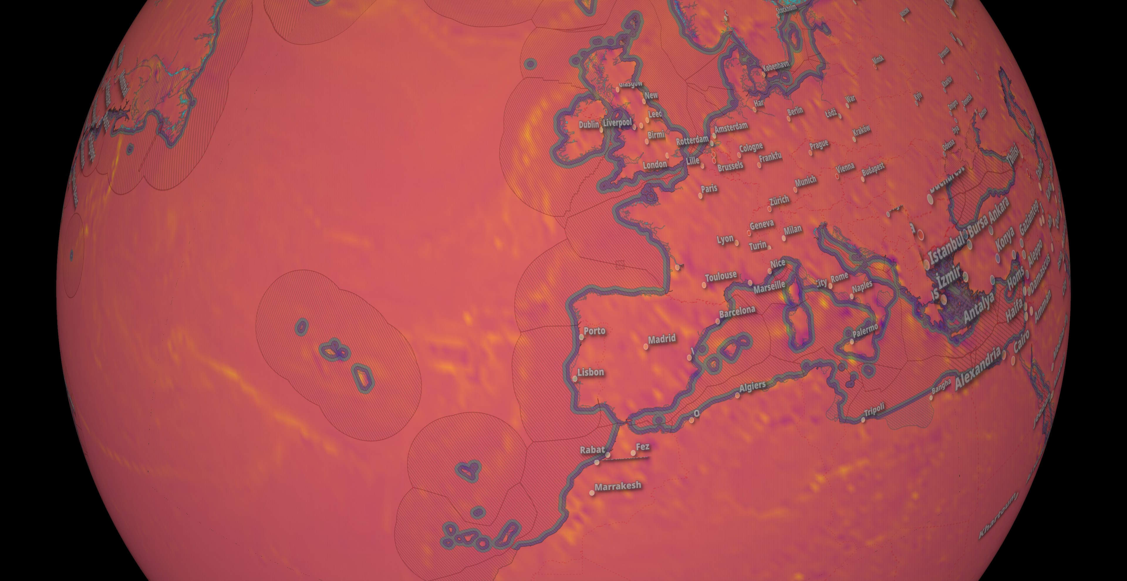
Each file has data covering the entire planet. These are the contents of gfs_4_20260501_1800_000.grb2 rendered on a globe in QGIS.
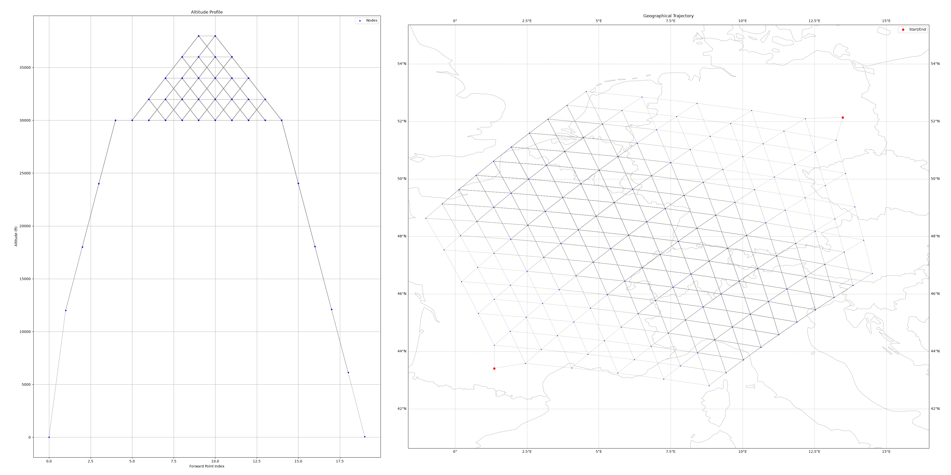
This is the solver's altitude and geographical search space.
plot_network_adapted(
    graph=domain.network,
    p0=LatLon(43.629444, 1.363056),
    p1=LatLon(
        airport("EDDB")["lat"],
        airport("EDDB")["lon"],
        airport("EDDB")["alt"] * ft))
This is the optimal flight path according to the solver.
solver = Astar(
            domain_factory=domain_factory,
            heuristic=lambda d, s: d.heuristic(s),
            parallel=False)

solver.solve()
A* finished to solve from state ... in 0.28 seconds
domain.custom_rollout(solver=solver, make_img=True)
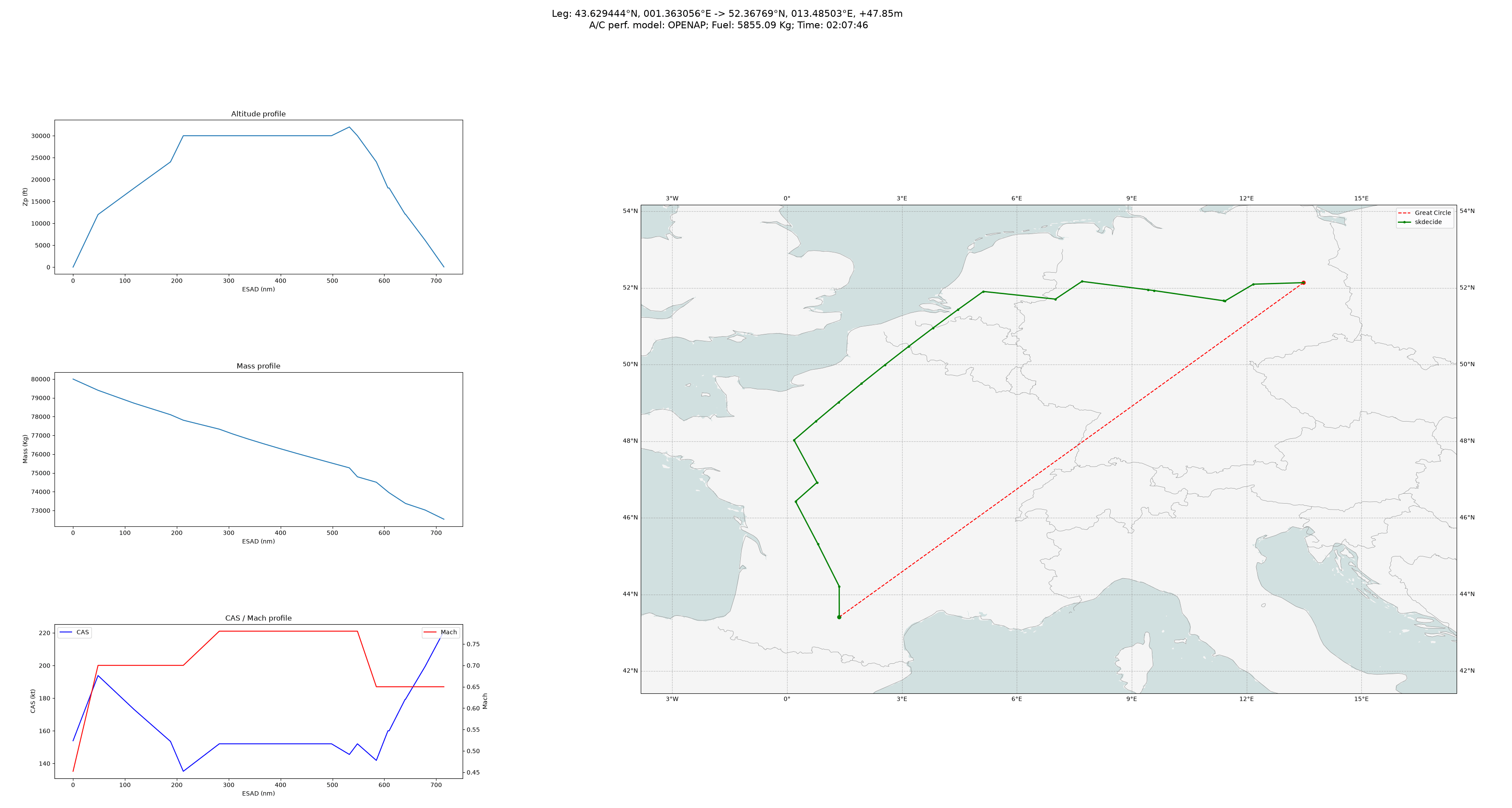
Goal reached after 19 steps!
({'time': 7666.281474928903, 'fuel': 5855.093906205222}, None)
I'll format each of the flight plan's steps so they're easier to read.
domain.observation.trajectory.to_csv('TLS-BER.csv', index=None)
$ ~/duckdb
SELECT   phase: UPPER(phase),
         time_: ts::INT,
         alt:   alt::INT,
         mass:  mass::INT,
         mach:  ROUND(mach, 2),
         cas:   cas::INT,
         fuel:  fuel::INT,
         geom:  ST_POINT(lon, lat)
FROM     'TLS-BER.csv'
ORDER BY ts;
┌─────────┬───────┬───────┬───────┬────────┬───────┬───────┬────────────────────────────────────────────────┐
│  phase  │ time_ │  alt  │ mass  │  mach  │  cas  │ fuel  │                      geom                      │
│ varchar │ int32 │ int32 │ int32 │ double │ int32 │ int32 │                    geometry                    │
├─────────┼───────┼───────┼───────┼────────┼───────┼───────┼────────────────────────────────────────────────┤
│ CLIMB   │ 28800 │     0 │ 80000 │   0.45 │   154 │     0 │ POINT (1.363056 43.629444)                     │
│ CLIMB   │ 29183 │ 12000 │ 79402 │    0.7 │   194 │   598 │ POINT (1.3614644301412264 44.431571122861556)  │
│ CLIMB   │ 29767 │ 18000 │ 78717 │    0.7 │   173 │   685 │ POINT (0.8028803270337778 45.54329961845038)   │
│ CLIMB   │ 30367 │ 24000 │ 78104 │    0.7 │   154 │     2 │ POINT (0.22308186850312028 46.64860136322122)  │
│ CLIMB   │ 30369 │ 24000 │ 78102 │    0.7 │   154 │     2 │ POINT (0.2213600223765711 46.65181397470445)   │
│ CLIMB   │ 30691 │ 30000 │ 77808 │    0.7 │   135 │   294 │ POINT (0.781910701674247 47.146798229437145)   │
│ CRUISE  │ 31222 │ 30000 │ 77331 │   0.78 │   152 │   477 │ POINT (0.18057649919536045 48.254448220756515) │
│ CRUISE  │ 31515 │ 30000 │ 77070 │   0.78 │   152 │   262 │ POINT (0.7571242215277763 48.74964861278412)   │
│ CRUISE  │ 31805 │ 30000 │ 76812 │   0.78 │   152 │   258 │ POINT (1.3446668642885302 49.24219441171162)   │
│ CRUISE  │ 32093 │ 30000 │ 76555 │   0.78 │   152 │   256 │ POINT (1.943586016571517 49.732000774167815)   │
│ CRUISE  │ 32382 │ 30000 │ 76298 │   0.78 │   152 │   257 │ POINT (2.554285524033502 50.218985517421046)   │
│ CRUISE  │ 32672 │ 30000 │ 76041 │   0.78 │   152 │   257 │ POINT (3.1771982015706532 50.70307279893911)   │
│ CRUISE  │ 32961 │ 30000 │ 75786 │   0.78 │   152 │   256 │ POINT (3.812797488711077 51.18419969012497)    │
│ CRUISE  │ 33252 │ 30000 │ 75529 │   0.78 │   152 │   257 │ POINT (4.461619033936127 51.66232853895605)    │
│ CRUISE  │ 33547 │ 32000 │ 75270 │   0.78 │   146 │   259 │ POINT (5.1243038676232 52.13747186609129)      │
│ CRUISE  │ 34103 │ 30000 │ 74794 │   0.78 │   152 │   476 │ POINT (7.006628090474678 51.93831668841654)    │
│ DESCENT │ 34458 │ 24031 │ 74503 │   0.65 │   142 │   290 │ POINT (7.7011825929472675 52.40044729715865)   │
│ DESCENT │ 35058 │ 18063 │ 73995 │   0.65 │   160 │    51 │ POINT (9.423199233939213 52.1821111144618)     │
│ DESCENT │ 35114 │ 18063 │ 73944 │   0.65 │   160 │    51 │ POINT (9.580613666598857 52.160789987133924)   │
│ DESCENT │ 35714 │ 12094 │ 73388 │   0.65 │   179 │    13 │ POINT (11.398384342445423 51.895274115132494)  │
│ DESCENT │ 35727 │ 12094 │ 73375 │   0.65 │   179 │    13 │ POINT (11.435080901553494 51.88959204464927)   │
│ DESCENT │ 36063 │  6126 │ 73023 │   0.65 │   199 │   352 │ POINT (12.17769156482302 52.32776873134525)    │
│ DESCENT │ 36466 │    48 │ 72534 │   0.65 │   221 │   488 │ POINT (13.48503 52.36769)                      │
└─────────┴───────┴───────┴───────┴────────┴───────┴───────┴────────────────────────────────────────────────┘
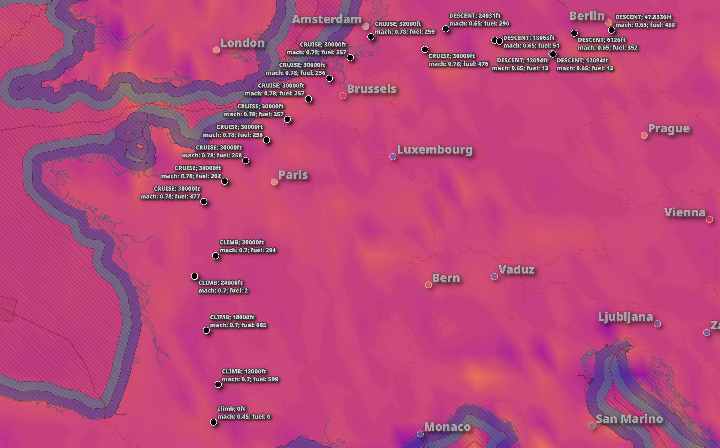
I'll export the flight plan to Parquet and render it on top of the ground-level wind data in QGIS.
COPY (
    SELECT   * EXCLUDE(lon, lat),
             geometry: ST_POINT(lon, lat)
    FROM     'TLS-BER.csv'
    ORDER BY ts
) TO 'TLS-BER.parquet' (
      FORMAT 'PARQUET',
      CODEC  'ZSTD',
      COMPRESSION_LEVEL 22,
      ROW_GROUP_SIZE 15000);
Toulouse to Warsaw
Below, I'll find an optimal flight path from Toulouse-Blagnac Airport (LFBO / TLS) to Warsaw Chopin Airport (EPWA / WAW).
The initial target altitude will be much higher than in the previous example. The result is a flight that is able to take a much more direct route.
acState = AircraftState(
    model_type="A320",
    performance_model_type=PerformanceModelEnum.OPENAP,
    gw_kg=80_000,
    zp_ft=18000.0,
    mach=cas2mach(250 * kts, h=10_000 * ft),
    phase=PhaseEnum.CLIMB,
    rating_level=RatingEnum.MCL,
    cg=0.3,
    x_graph=5,
    y_graph=5,
    z_graph=10)

domain_factory = lambda: FlightPlanningDomain(
    aircraft_state=acState,
    mach_cruise=0.78,
    mach_climb=0.7,
    mach_descent=0.65,
    nb_forward_points=20,
    nb_lateral_points=10,
    nb_climb_descent_steps=5,
    flight_levels_ft=list(np.arange(30_000, 38_000 + 2_000, 2_000)),
    graph_width="medium",
    origin=LatLon(43.629444, 1.363056),
    destination="EPWA",
    objective=cost_function,
    heuristic_name=heuristic,
    weather_date=weather_date)

domain = domain_factory()

solver = Astar(
            domain_factory=domain_factory,
            heuristic=lambda d, s: d.heuristic(s),
            parallel=False)

solver.solve()
A* finished to solve from state ... in 29.45 seconds.
domain.custom_rollout(solver=solver, make_img=True)
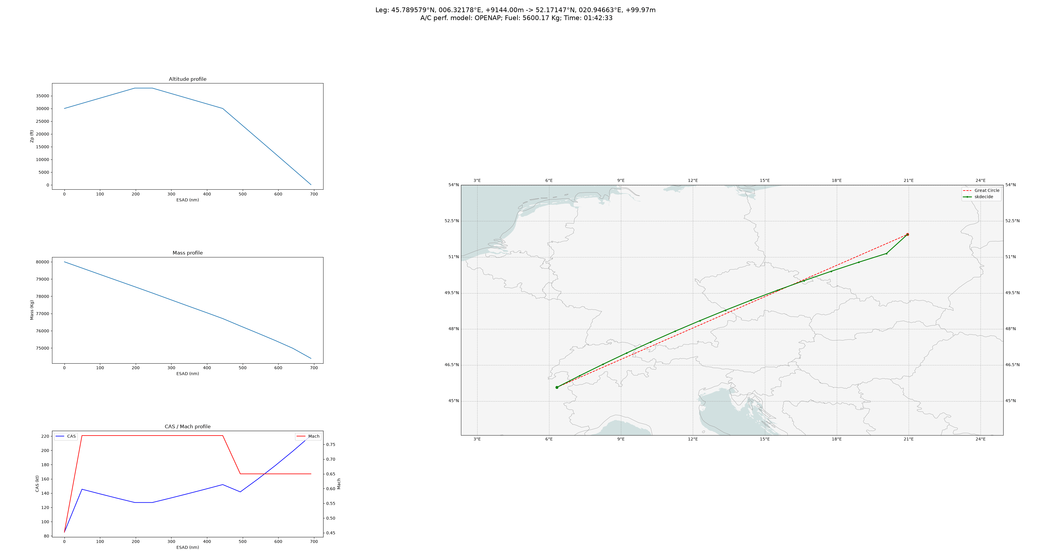
Goal reached after 14 steps!
({'time': 6153.660431613251, 'fuel': 5600.171145693044}, None)
Warsaw is 500 KM further away from Toulouse than Berlin. But the faster climb to cruising altitude under the given wind conditions meant the aircraft could take a more direct route. It made it to Warsaw almost 45 minutes faster and only needed 76% of the fuel that the Berlin flight needed.
These are the steps in the above flight plan.
domain.observation.trajectory.to_csv('TLS-WAW.csv', index=None)
$ ~/duckdb
SELECT   phase: UPPER(phase),
         time_: ts::INT,
         alt:   alt::INT,
         mass:  mass::INT,
         mach:  ROUND(mach, 2),
         cas:   cas::INT,
         fuel:  fuel::INT,
         geom:  ST_POINT(lon, lat)
FROM     'TLS-WAW.csv'
ORDER BY ts;
┌─────────┬───────┬───────┬───────┬────────┬───────┬───────┬───────────────────────────────────────────────┐
│  phase  │ time_ │  alt  │ mass  │  mach  │  cas  │ fuel  │                     geom                      │
│ varchar │ int32 │ int32 │ int32 │ double │ int32 │ int32 │                   geometry                    │
├─────────┼───────┼───────┼───────┼────────┼───────┼───────┼───────────────────────────────────────────────┤
│ CLIMB   │ 28800 │ 30000 │ 80000 │   0.45 │    85 │     0 │ POINT (6.321780309765473 45.78957852956533)   │
│ CRUISE  │ 29196 │ 32000 │ 79639 │   0.78 │   146 │   361 │ POINT (7.274006698354081 46.275553205520794)  │
│ CRUISE  │ 29604 │ 34000 │ 79276 │   0.78 │   139 │   363 │ POINT (8.243146568075773 46.75332543362598)   │
│ CRUISE  │ 30018 │ 36000 │ 78915 │   0.78 │   133 │   361 │ POINT (9.229481862337197 47.22261290149568)   │
│ CRUISE  │ 30436 │ 38000 │ 78555 │   0.78 │   127 │   360 │ POINT (10.23327610333648 47.68312559281413)   │
│ CRUISE  │ 30861 │ 38000 │ 78191 │   0.78 │   127 │   365 │ POINT (11.25477083484032 48.13456566890824)   │
│ CRUISE  │ 31297 │ 36000 │ 77819 │   0.78 │   133 │   371 │ POINT (12.29418112454121 48.57662718213212)   │
│ CRUISE  │ 31732 │ 34000 │ 77449 │   0.78 │   139 │   370 │ POINT (13.351689351409924 49.00899540355703)  │
│ CRUISE  │ 32161 │ 32000 │ 77082 │   0.78 │   146 │   367 │ POINT (14.427435465032865 49.431345252175966) │
│ CRUISE  │ 32589 │ 30000 │ 76710 │   0.78 │   152 │   372 │ POINT (15.521498988740307 49.843337488922174) │
│ DESCENT │ 33101 │ 24066 │ 76280 │   0.65 │   142 │   429 │ POINT (16.633858546975723 50.2446086742223)   │
│ DESCENT │ 33589 │ 18131 │ 75861 │   0.65 │   160 │   420 │ POINT (17.764276668345886 50.63474030548783)  │
│ DESCENT │ 34046 │ 12197 │ 75433 │   0.65 │   179 │   428 │ POINT (18.91184798374883 51.01313503252613)   │
│ DESCENT │ 34472 │  6262 │ 74984 │   0.65 │   199 │   449 │ POINT (20.071843186874247 51.378167839584854) │
│ DESCENT │ 34954 │   100 │ 74400 │   0.65 │   221 │   584 │ POINT (20.94663 52.17147)                     │
└─────────┴───────┴───────┴───────┴────────┴───────┴───────┴───────────────────────────────────────────────┘
Airbus A320 vs Boeing 737
OpenTop can be paired with OpenAP and used to figure out flight trajectories between two airports.
Its optimiser requires a grid cost file. I'll first download an example 142 MB NetCDF file provided by the project.
$ wget https://opendap.4tu.nl/thredds/fileServer/data2/djht/bea8a3fe-e34c-4598-9f94-c5a5c63348e5/1/contrail_original.nc
The cost file can be either in Casadi or Parquet format. I worked from an example in its documentation, which produced a 246 KB Casadi file.
import openap
import pandas as pd
from scipy.ndimage import gaussian_filter
from opentop.tools import cached_interpolant_from_dataframe
import xarray as xr

ds = xr.open_dataset('contrail_original.nc')\
       .sel(time='2015-12-18')

level_pressure = [
    0.0000,
    10.0000,
    30.0000,
    50.0000,
    70.0000,
    90.0787,
    110.6606,
    132.3968,
    155.7909,
    181.1544,
    208.6494,
    238.3258,
    270.1530,
    304.0465,
    339.8891,
    377.5467,
    416.8789,
    457.7442,
    500.0000,
    543.4970,
    588.0685,
    633.5144,
    679.5799,
    725.9285,
    772.1102,
    817.5241,
    861.3757,
    902.6287,
    939.9520,
    971.6610,
    995.6532,
    1009.3396]

df = (
    ds.to_dataframe()
    .reset_index()
    .assign(lev=lambda x: x.lev.astype(int))
    .merge(
        pd.DataFrame(level_pressure, columns=["hPa"]).reset_index(names="lev"),
        on="lev",
    )
    .assign(height=lambda x: openap.aero.h_isa(x.hPa * 100).round(-2))
    .assign(longitude=lambda x: ((x.lon + 180) % 360 - 180))
    .query("height<15000"))

df_cost_world = df.rename(
    columns={
        "lat": "latitude",
        "atr20_contrail": "cost",
    }
)[["time",
   "latitude",
   "longitude",
   "hPa",
   "height",
   "cost"]]


df_cost = df_cost_world.query(
    "-20<longitude<40 and 30<latitude<70 and time.dt.hour==12"
).sort_values(["height", "latitude", "longitude"])

cost = df_cost.cost.values.reshape(
    df_cost.height.nunique(),
    df_cost.latitude.nunique(),
    df_cost.longitude.nunique())

cost_ = gaussian_filter(cost, sigma=1, mode="nearest")
df_cost = df_cost.assign(cost=cost_.flatten())

interpolant = cached_interpolant_from_dataframe(
                df_cost,
                "contrail.casadi",
                shape="bspline")
These are the first and last few bytes of its contents.
$ hexdump -C contrail.casadi | head
00000000  6a 68 70 6e 6e 61 67 69  69 65 61 68 61 61 61 61  |jhpnnagiieahaaaa|
00000010  64 61 61 61 61 61 61 61  61 61 61 61 61 61 61 61  |daaaaaaaaaaaaaaa|
00000020  61 61 66 61 65 67 61 61  6c 61 61 61 61 61 61 61  |aafaegaalaaaaaaa|
00000030  6a 65 6f 67 65 68 66 67  63 68 61 68 70 67 6d 67  |jeogehfgchahpgmg|
00000040  62 67 6f 67 65 68 68 61  61 61 61 61 61 61 63 67  |bgogehhaaaaaaacg|
00000050  64 68 61 68 6d 67 6a 67  6f 67 66 67 63 61 61 61  |dhahmgjgogfgcaaa|
00000060  61 61 61 61 6a 61 61 61  61 61 61 61 68 67 63 68  |aaaajaaaaaaahgch|
00000070  6a 67 65 67 70 66 64 67  70 67 64 68 65 68 61 61  |jgegpfdgpgdhehaa|
00000080  61 61 61 61 61 61 62 61  69 61 61 61 61 61 61 61  |aaaaaabaiaaaaaaa|
00000090  62 61 61 61 61 61 61 61  61 61 61 61 61 61 61 61  |baaaaaaaaaaaaaaa|
$ hexdump -C contrail.casadi | tail
0003d620  61 61 61 61 61 61 64 62  61 61 61 61 61 61 61 61  |aaaaaadbaaaaaaaa|
0003d630  61 61 61 61 61 61 67 62  61 61 61 61 61 61 61 61  |aaaaaagbaaaaaaaa|
0003d640  61 61 61 61 61 61 68 62  61 61 61 61 61 61 61 61  |aaaaaahbaaaaaaaa|
0003d650  61 61 61 61 61 61 61 61  61 61 61 61 61 61 61 61  |aaaaaaaaaaaaaaaa|
0003d660  61 61 61 61 61 61 62 61  61 61 61 61 61 61 61 61  |aaaaaabaaaaaaaaa|
0003d670  61 61 61 61 61 61 61 61  61 61 61 61 61 61 61 61  |aaaaaaaaaaaaaaaa|
0003d680  61 61 61 61 61 61 62 61  61 61 62 61 61 61 61 61  |aaaaaabaaabaaaaa|
0003d690  61 61 61 61 61 61 61 61  61 61 63 68 67 61 61 61  |aaaaaaaaaachgaaa|
0003d6a0  61 61 61 61 61 61 61 61  61 61 61 61              |aaaaaaaaaaaa|
0003d6ac
I noticed the contents are repetitive and compress well.
$ gzip -9 < contrail.casadi | wc -c
90949
I'll get the metrics of an optimal flight between Amsterdam's Schiphol (EHAM / AMS) and Frankfurt (EDDF / FRA) on an Airbus A320.
$ opentop optimize \
    EHAM EDDF \
    -a A320 \
    --phase all \
    --obj "0.3*fuel+0.7*grid" \
    --grid contrail.casadi
aircraft:  A320
route:     EHAM → EDDF
phase:     all
objective: 0.3*fuel+0.7*grid
m0:        0.85
max_iter:  1500
grid file: contrail.casadi

success:       True
return_status: Solve_Succeeded
iter_count:    179
wall time:     12.2 s
objective:     4.8768e+02
fuel burn:     1625.6 kg
max altitude:  19891 ft
flight time:   35.8 min
I'll then do the same using a Boeing 737.
$ opentop optimize \
    EHAM EDDF \
    -a B737 \
    --phase all \
    --obj "0.3*fuel+0.7*grid" \
    --grid contrail.casadi
aircraft:  B737
route:     EHAM → EDDF
phase:     all
objective: 0.3*fuel+0.7*grid
m0:        0.85
max_iter:  1500
grid file: contrail.casadi

success:       True
return_status: Solve_Succeeded
iter_count:    141
wall time:     9.9 s
objective:     4.8662e+02
fuel burn:     1622.1 kg
max altitude:  21968 ft
flight time:   39.2 min