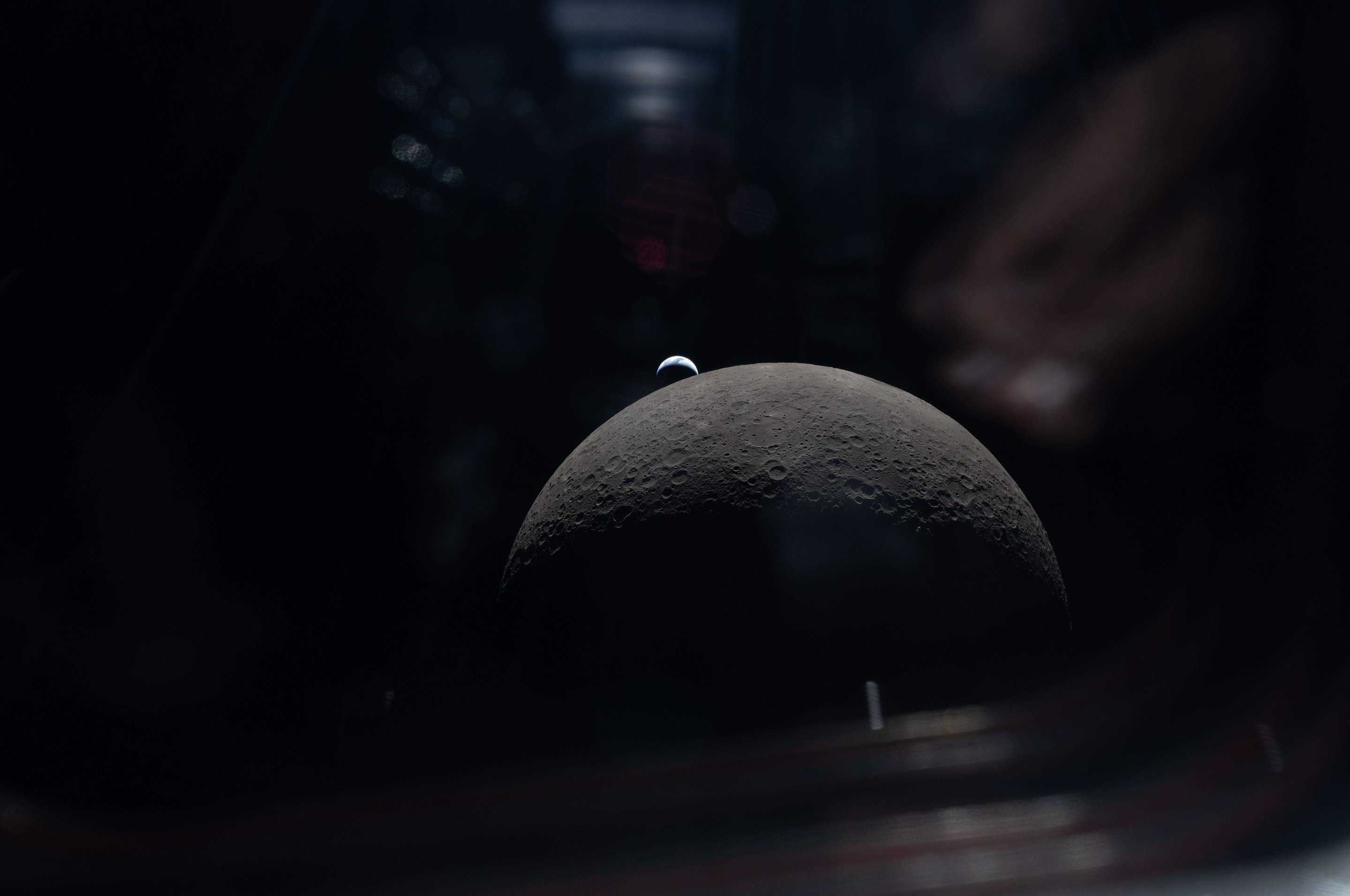
In April, NASA sent four astronauts on a flyby mission around the Moon. They've since published 12,217 JPEGs that were captured during the 9-day journey.
In this post, I'll attempt to categorise the imagery and analyse the accompanying metadata.
My Workstation
I'm using a 5.7 GHz AMD Ryzen 9 9950X CPU. It has 16 cores and 32 threads and 1.2 MB of L1, 16 MB of L2 and 64 MB of L3 cache. It has a liquid cooler attached and is housed in a spacious, full-sized Cooler Master HAF 700 computer case.
The system has 96 GB of DDR5 RAM clocked at 4,800 MT/s and a 5th-generation, Crucial T700 4 TB NVMe M.2 SSD which can read at speeds up to 12,400 MB/s. There is a heatsink on the SSD to help keep its temperature down. This is my system's C drive.
The system is powered by a 1,200-watt, fully modular Corsair Power Supply and is sat on an ASRock X870E Nova 90 Motherboard.
I'm running Ubuntu 24 LTS via Microsoft's Ubuntu for Windows on Windows 11 Pro. In case you're wondering why I don't run a Linux-based desktop as my primary work environment, I'm still using an Nvidia GTX 1080 GPU which has better driver support on Windows and ArcGIS Pro only supports Windows natively.
Installing Prerequisites
I'll use Python 3.12.3 and a few other tools to help analyse the data in this post.
$ sudo add-apt-repository ppa:deadsnakes/ppa
$ sudo add-apt-repository ppa:ubuntugis/ubuntugis-unstable
$ sudo apt update
$ sudo apt install \
    jq \
    libimage-exiftool-perl \
    python3-pip \
    python3.12-venv
I'll be using JSON Convert (jc) to convert the output of various CLI tools into JSON.
$ wget https://github.com/kellyjonbrazil/jc/releases/download/v1.25.2/jc_1.25.2-1_amd64.deb
$ sudo dpkg -i jc_1.25.2-1_amd64.deb
I'll set up a Python Virtual Environment and install a few dependencies needed to run one of OpenAI's models on NASA's imagery.
$ python3 -m venv ~/.nasa_artemis
$ source ~/.nasa_artemis/bin/activate
$ python3 -m pip install \
    'pillow==10.4.0' \
    rich \
    transformers
I'll be using a Python-based image contact sheet generator in this post.
$ git clone https://github.com/cobanov/contact-sheet \
    ~/contact-sheet

$ pip install -r \
    ~/contact-sheet/requirements.txt
I'll use DuckDB, along with its H3, JSON, Lindel, Parquet and Spatial extensions in this post.
$ cd ~
$ wget -c https://github.com/duckdb/duckdb/releases/download/v1.5.1/duckdb_cli-linux-amd64.zip
$ unzip -j duckdb_cli-linux-amd64.zip
$ chmod +x duckdb
$ ~/duckdb
INSTALL h3 FROM community;
INSTALL lindel FROM community;
INSTALL json;
INSTALL parquet;
INSTALL spatial;
I'll set up DuckDB to load every installed extension each time it launches.
$ vi ~/.duckdbrc
.timer on
.width 180
LOAD h3;
LOAD lindel;
LOAD json;
LOAD parquet;
LOAD spatial;
Downloading 12K+ JPEGs
I'll create a folder for the contents of this post.
$ mkdir -p ~/artemis2
$ cd ~/artemis2
NASA lists and serves the images on a Perl-based portal. I had to copy the list of image IDs and paste them into a text file.
The file contains 12,217 lines.
$ wc -l manifest.txt # 12217
Below are a few example lines.
$ sort -R manifest.txt | head
ART002-E-20055
ART002-E-29232
ART002-E-11714
ART002-E-24812
ART002-E-23347
ART002-E-29751
ART002-E-11580
ART002-E-26846
ART002-E-20928
ART002-E-10963
I used Python to generate a BASH file containing wget commands to download each image.
$ python3
from pathlib import Path


with open('run.bash', 'w') as f:
    for line in open('manifest.txt'):
        id_ = int(line.split('-')[2])

        if not Path("%d.JPG" % id_).is_file():
            f.write("wget -c -O \"%d.JPG\" \"https://eol.jsc.nasa.gov/DatabaseImages/ESC/large/ART002/ART002-E-%d.JPG\"\n" % (id_, id_))
The following will run 16 concurrent downloads from the above BASH script.
$ cat run.bash \
    | xargs -n1 \
            -P16 \
            -I% \
            bash -c "%"
Some of the downloads failed for one reason or another. I ran the following to remove any 0-byte files. Following that, I regenerated the BASH script and re-ran it to try and see if any more images could be downloaded.
$ find . \
       -type f \
       -size 0 \
       -print0 \
    | xargs \
        -I{} \
        -0 \
        rm {}
I was able to download a total of 11,362 JPEGs totalling 14 GB altogether. 885 images are still outstanding.
$ ls *.JPG | wc -l # 11362
$ du -hsc *.JPG | tail -n1 # 14 GB
Extracting EXIF Metadata
Below, I've extracted the EXIF metadata from each image into its own JSON-formatted line.
$ touch metadata.json; rm metadata.json

$ for FILENAME in *.JPG; do
      exiftool $FILENAME \
        | jc --kv \
        | jq -Sc . \
        >> metadata.json
  done
I usually import JSON files directly into DuckDB but the JSONL files have at least 7 or 8 different schemas. DuckDB will only import these as a single JSON map column instead of as a few-hundred-column table.
To get around this, I cherry-picked columns with keywords in their names and produced a resulting JSONL file with far fewer columns.
$ python3
import json


keywords = (
    'aperture',
    'exposure',
    'focal',
    'shutter',
    'camera',
    'lens',
    'date',
    'time',
)

with open('metadata.cleaned.json', 'w') as f:
    for line in open('metadata.json'):
        f.write(
            json.dumps(
                {k.lower().replace(' ', '_'): v
                 for k, v in json.loads(line).items()
                 if any(True
                        for keyword in keywords
                        if keyword.lower() in k.lower() or
                           k.lower() == 'file name')},
                sort_keys=True,
                default=str) + '\n')
Below is a breakdown of unique values and NULL coverage across each column. I've excluded columns with fewer than two unique values and a few with very long names that I'm not interested in.
$ ~/duckdb
.maxrows 100

SELECT   column_name,
         null_percentage,
         approx_unique,
         min[:30],
         max[:30]
FROM     (SUMMARIZE
          FROM 'metadata.cleaned.json')
WHERE    approx_unique > 1
AND      column_name NOT LIKE '%param%'
AND      column_name NOT LIKE '%perspective_model_scale_factor%'
ORDER BY LOWER(column_name);
┌──────────────────────────────────┬─────────────────┬───────────────┬────────────────────────────────┬────────────────────────────────┐
│           column_name            │ null_percentage │ approx_unique │            min[:30]            │            max[:30]            │
│             varchar              │  decimal(9,2)   │     int64     │            varchar             │            varchar             │
├──────────────────────────────────┼─────────────────┼───────────────┼────────────────────────────────┼────────────────────────────────┤
│ aperture                         │           11.34 │            22 │ 1.2                            │ 9.0                            │
│ aperture_value                   │           11.34 │            22 │ 1.2                            │ 9.0                            │
│ camera_model_name                │           11.34 │             2 │ NIKON D5                       │ NIKON Z 9                      │
│ camera_profile                   │           11.34 │             2 │ Adobe Standard                 │ Camera Standard                │
│ camera_profile_digest            │           11.34 │             4 │ 69725A6B5714B6777D9E68B8C0DC18 │ EF370D7B22F72601AB8DD41D8D45B0 │
│ camera_profiles_aperture_value   │           75.55 │            11 │ 2                              │ 8.918863                       │
│ camera_profiles_focal_length     │           75.55 │            18 │ 125                            │ 98                             │
│ camera_profiles_lens             │           75.55 │             3 │ 14-24mm f/2.8G                 │ VR 80-400mm f/4.5-5.6G         │
│ camera_profiles_lens_pretty_name │           75.55 │             3 │ 14-24mm f/2.8G                 │ VR 80-400mm f/4.5-5.6G         │
│ create_date                      │            0.00 │         11150 │ 2025:09:19 15:24:02.62         │ 2026:04:13 08:03:42-05:00      │
│ date/time_created                │            0.00 │          5515 │ 2025:09:19 15:24:02            │ 2026:04:13 08:03:42-05:00      │
│ date/time_original               │            0.00 │         11150 │ 2025:09:19 15:24:02.62         │ 2026:04:13 08:03:42-05:00      │
│ date_created                     │            0.00 │         11459 │ 2025:09:19 15:24:02.62         │ 2026:04:13 08:03:42-05:00      │
│ digital_creation_date            │            0.00 │            12 │ 2025:09:19                     │ 2026:04:13                     │
│ digital_creation_date/time       │            0.00 │          5166 │ 2025:09:19 15:24:02            │ 2026:04:13 08:03:42-05:00      │
│ digital_creation_time            │            0.00 │          3863 │ 00:04:19                       │ 23:59:18+00:00                 │
│ exposure_compensation            │           11.34 │            17 │ +1                             │ 0                              │
│ exposure_mode                    │           11.34 │             2 │ Auto                           │ Manual                         │
│ exposure_program                 │           11.34 │             2 │ Manual                         │ Program AE                     │
│ exposure_time                    │           11.34 │            53 │ 0.3                            │ 8                              │
│ file_access_date/time            │            0.00 │          1701 │ 2026:05:07 20:12:53+03:00      │ 2026:05:08 11:48:34+03:00      │
│ file_inode_change_date/time      │            0.00 │          3308 │ 2026:05:07 18:46:56+03:00      │ 2026:05:08 11:48:34+03:00      │
│ file_modification_date/time      │            0.00 │          2177 │ 2026:04:22 20:29:35+03:00      │ 2026:04:22 21:30:07+03:00      │
│ file_name                        │            0.00 │         11567 │ 10000.JPG                      │ 9999.JPG                       │
│ focal_length                     │           11.34 │            61 │ 100.0 mm (35 mm equivalent: 10 │ 98.0 mm (35 mm equivalent: 98. │
│ focal_length_in_35mm_format      │           11.34 │            50 │ 100 mm                         │ 98 mm                          │
│ focal_plane_x_resolution         │           11.34 │             2 │ 1552.056122                    │ 2301.324615                    │
│ focal_plane_y_resolution         │           11.34 │             2 │ 1552.056122                    │ 2301.324615                    │
│ hyperfocal_distance              │           11.34 │           410 │ 0.47 m                         │ 99.95 m                        │
│ lens                             │           11.34 │             5 │ 0.0 mm f/0.0                   │ VR 80-400mm f/4.5-5.6G         │
│ lens_id                          │           11.34 │             6 │ 0.0mm f/0.0                    │ VR 80-400mm f/4.5-5.6G         │
│ lens_info                        │           11.34 │             3 │ 0mm f/0                        │ 80-400mm f/4.5-5.6             │
│ lens_model                       │           11.34 │             5 │ 0.0 mm f/0.0                   │ VR 80-400mm f/4.5-5.6G         │
│ lens_profile_digest              │           78.59 │            76 │ 0084F848238B2AD219A96E222F8145 │ FC43CB862288DC032EBB3109258565 │
│ lens_profile_enable              │            0.00 │             2 │ 0                              │ 1                              │
│ max_aperture_value               │           35.79 │            10 │ 1.0                            │ 5.7                            │
│ metadata_date                    │            0.00 │          7217 │ 2026:04:03 04:25:44-05:00      │ 2026:04:21 17:31:25-05:00      │
│ modify_date                      │            0.00 │          7217 │ 2026:04:03 04:25:44-05:00      │ 2026:04:21 17:31:25-05:00      │
│ offset_time_digitized            │           64.22 │             2 │ +00:00                         │ -05:00                         │
│ recommended_exposure_index       │           11.34 │            23 │ 1000                           │ 8000                           │
│ shutter_speed                    │           11.34 │            53 │ 0.3                            │ 8                              │
│ shutter_speed_value              │           11.34 │            53 │ 0.3                            │ 8                              │
│ sub_sec_time_digitized           │           11.34 │            90 │ 00                             │ 99                             │
│ sub_sec_time_original            │           11.34 │            90 │ 00                             │ 99                             │
│ time_created                     │            0.00 │          3547 │ 00:04:19                       │ 23:59:18                       │
└──────────────────────────────────┴─────────────────┴───────────────┴────────────────────────────────┴────────────────────────────────┘
Image Classification
Below, I'll run each JPEG through a zero-shot image classifier OpenAI released a few years ago. I've given the model five classification labels to choose from.
I randomised the order of the images to assist with spot-checking the results during the hour it took to run.
$ python3
import json
from   glob import glob
import random

from PIL           import Image
from rich.progress import track
from transformers  import pipeline


detector  = pipeline(model='openai/clip-vit-large-patch14',
                     task='zero-shot-image-classification')
labels    = ['earth', 'moon', 'stars', 'blank', 'glare']

filenames = list(glob('*.JPG'))
random.shuffle(filenames)

with open('classifications.json', 'w') as f:
    for filename in track(filenames):
        resp = detector(Image.open(filename),
                        candidate_labels=labels)
        top_res = sorted(resp,
                         key=lambda x: x['score'],
                         reverse=True)[0]
        resp = {'filename': filename,
                'label':    top_res['label'],
                'score':    top_res['score']}
        f.write(json.dumps(resp, sort_keys=True) + '\n')
Joining Datasets
I'll import the camera EXIF metadata along with the classifications above into DuckDB and join them into a single table.
$ ~/duckdb nasa.duckdb
CREATE OR REPLACE TABLE classifications AS
    FROM 'classifications.json';

CREATE OR REPLACE TABLE camera_settings AS
    FROM 'metadata.cleaned.json';

CREATE OR REPLACE TABLE imagery AS
    FROM classifications c
    JOIN camera_settings s ON c.filename = s.file_name;
Contact Sheets
Below are the number of imges for each label.
$ ~/duckdb nasa.duckdb
SELECT   COUNT(*),
         label
FROM     imagery
GROUP BY 2
ORDER BY 1 DESC;
┌──────────────┬─────────┐
│ count_star() │  label  │
│    int64     │ varchar │
├──────────────┼─────────┤
│         7028 │ moon    │
│         1490 │ stars   │
│         1250 │ earth   │
│         1030 │ blank   │
│          564 │ glare   │
└──────────────┴─────────┘
I'll generate a contact sheet for each classification label.
$ for LABEL in blank earth moon stars glare; do
      echo "SELECT filename
            FROM   classifications
            WHERE  label = '$LABEL'" \
          | ~/duckdb -list -noheader nasa.duckdb \
          > "${LABEL}.txt"
      python3 ~/contact-sheet/contact_sheet.py \
              --file_list "${LABEL}.txt" \
              "thumbnails.${LABEL}.jpeg"
  done
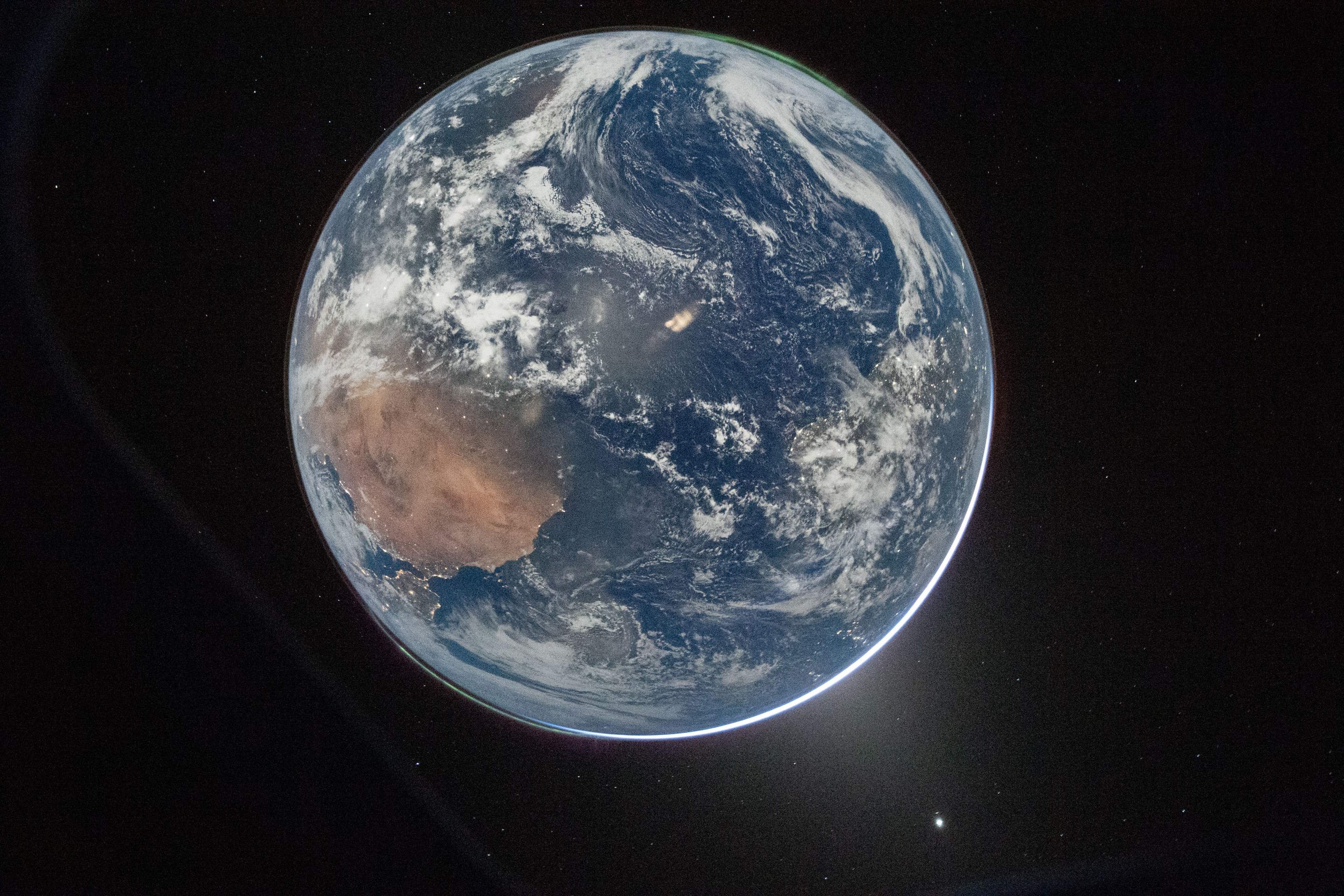
These are thumbnails of the images that the above model labelled as the Earth.

These are thumbnails of the images that the above model labelled as the Moon.

These are thumbnails of the images that the above model labelled as stars.

These are thumbnails of the images that the above model labelled as glare.

These are thumbnails of the images that the above model labelled as being blank.

Below are the image counts for each score bins for each label.
$ ~/duckdb nasa.duckdb
WITH a AS (
    SELECT   label,
             score_bin: ROUND(score, 1),
             num_pics:  COUNT(*)
    FROM     imagery
    GROUP BY 1, 2
)
PIVOT    a
ON       label,
USING    SUM(num_pics)
GROUP BY score_bin
ORDER BY score_bin;
┌───────────┬────────┬────────┬────────┬────────┬────────┐
│ score_bin │ blank  │ earth  │ glare  │  moon  │ stars  │
│  double   │ int128 │ int128 │ int128 │ int128 │ int128 │
├───────────┼────────┼────────┼────────┼────────┼────────┤
│       0.2 │   NULL │   NULL │   NULL │   NULL │      1 │
│       0.3 │     76 │     12 │     22 │    115 │    101 │
│       0.4 │    188 │     19 │    131 │    237 │    538 │
│       0.5 │    157 │     43 │    145 │    201 │    480 │
│       0.6 │    596 │     48 │     91 │    145 │     63 │
│       0.7 │     13 │     35 │     75 │    115 │     20 │
│       0.8 │   NULL │     44 │     52 │    108 │     42 │
│       0.9 │   NULL │    115 │     37 │    239 │    154 │
│       1.0 │   NULL │    934 │     11 │   5868 │     91 │
└───────────┴────────┴────────┴────────┴────────┴────────┘
Spain at Night
The following is 192.JPG. Spain can be seen in the bottom left of the Earth's surface with its southern coast pointing upward. The Sun appears to illuminate the Earth from behind and the city lights all around Spain's coast and Madrid are clearly visible.
This is the metadata for this image.
$ echo "SELECT COLUMNS(c -> c NOT LIKE '%profiles%')
        FROM   imagery
        WHERE  file_name = '192.JPG'
        LIMIT  1" \
    | ~/duckdb -json nasa.duckdb 2>&1 \
    | grep '{.*' \
    | tail -c+6 \
    | jq -S .
[
  {
    "aperture": "4.0",
    "aperture_value": "4.0",
    "camera_model_name": "NIKON D5",
    "camera_profile": "Adobe Standard",
    "camera_profile_digest": "DC0173EBB7ECE22257A40AD42B5C9460",
    "create_date": "2026:04:03 00:27:39.26",
    "date/time_created": "2026:04:03 00:27:39",
    "date/time_original": "2026:04:03 00:27:39.26",
    "date_created": "2026:04:03 00:27:39.26",
    "digital_creation_date": "2026:04:03",
    "digital_creation_date/time": "2026:04:03 00:27:39",
    "digital_creation_time": "00:27:39",
    "exposure_2012": "0.00",
    "exposure_compensation": "+1",
    "exposure_mode": "Manual",
    "exposure_program": "Manual",
    "exposure_time": "1/4",
    "file_access_date/time": "2026:05:08 10:57:40+03:00",
    "file_inode_change_date/time": "2026:05:07 18:47:47+03:00",
    "file_modification_date/time": "2026:04:22 20:29:40+03:00",
    "file_name": "192.JPG",
    "filename": "192.JPG",
    "focal_length": "22.0 mm (35 mm equivalent: 22.0 mm)",
    "focal_length_in_35mm_format": "22 mm",
    "focal_plane_resolution_unit": "cm",
    "focal_plane_x_resolution": "1552.056122",
    "focal_plane_y_resolution": "1552.056122",
    "hyperfocal_distance": "4.03 m",
    "label": "earth",
    "lens": "14.0-24.0 mm f/2.8",
    "lens_id": "AF-S Zoom-Nikkor 14-24mm f/2.8G ED",
    "lens_info": "14-24mm f/2.8",
    "lens_manual_distortion_amount": "0",
    "lens_model": "14.0-24.0 mm f/2.8",
    "lens_profile_digest": null,
    "lens_profile_distortion_scale": null,
    "lens_profile_enable": "0",
    "lens_profile_is_embedded": null,
    "lens_profile_name": null,
    "lens_profile_setup": null,
    "lens_profile_vignetting_scale": null,
    "look_parameters_camera_profile": "Adobe Standard",
    "max_aperture_value": "2.8",
    "metadata_date": "2026:04:03 06:54:26-05:00",
    "modify_date": "2026:04:03 06:54:26-05:00",
    "offset_time": "-05:00",
    "offset_time_digitized": null,
    "offset_time_original": null,
    "profile_date_time": "1998:02:09 06:49:00",
    "recommended_exposure_index": "51200",
    "score": 0.9894962906837463,
    "shutter_speed": "1/4",
    "shutter_speed_value": "1/4",
    "sub_sec_time_digitized": "26",
    "sub_sec_time_original": "26",
    "time_created": "00:27:39"
  }
]
My guess from the sea of timestamps above is that this image was taken at 2026-04-03 00:27:39 UTC which would be 02:27:39 AM local time on the Spanish mainland.
The exposure time was only 1/4th of a second which normally isn't enough for any nighttime photography but the Nikon D5 camera this image was taken with supports an ISO of 51200. This level will make any dark scene very grainy but it ended up being a good trade-off in this case.
Settings and Timestamps
Below are the image counts per day by camera model.
$ ~/duckdb nasa.duckdb
WITH a AS (
    SELECT   camera_model_name,
             created_at: REPLACE(create_date[:10], ':', '-')::DATE,
             num_pics: COUNT(*)
    FROM     imagery
    GROUP BY 1, 2
)
PIVOT    a
ON       camera_model_name
USING    SUM(num_pics)
GROUP BY created_at
ORDER BY 1;
┌────────────┬──────────┬───────────┐
│ created_at │ NIKON D5 │ NIKON Z 9 │
│    date    │  int128  │  int128   │
├────────────┼──────────┼───────────┤
│ 2025-09-19 │        1 │      NULL │
│ 2026-04-02 │      629 │      NULL │
│ 2026-04-03 │      315 │        17 │
│ 2026-04-04 │       77 │      NULL │
│ 2026-04-05 │      160 │       149 │
│ 2026-04-06 │     4606 │      1689 │
│ 2026-04-07 │     1430 │       871 │
│ 2026-04-08 │       37 │        17 │
│ 2026-04-09 │       32 │        35 │
│ 2026-04-10 │        9 │      NULL │
│ 2026-04-13 │     NULL │      NULL │
└────────────┴──────────┴───────────┘
These are the lens counts.
WITH a AS (
    SELECT   camera_model_name,
             lens,
             num_pics: COUNT(*)
    FROM     imagery
    WHERE    camera_model_name IS NOT NULL
    GROUP BY 1, 2
)
PIVOT    a
ON       camera_model_name
USING    SUM(num_pics)
GROUP BY lens
ORDER BY 2 DESC;
┌─────────────────────────┬──────────┬───────────┐
│          lens           │ NIKON D5 │ NIKON Z 9 │
│         varchar         │  int128  │  int128   │
├─────────────────────────┼──────────┼───────────┤
│ 80.0-400.0 mm f/4.5-5.6 │     6987 │      NULL │
│ 14.0-24.0 mm f/2.8      │      246 │      NULL │
│ 35.0 mm f/2.0           │       62 │      NULL │
│ 0.0 mm f/0.0            │        1 │      NULL │
│ VR 80-400mm f/4.5-5.6G  │     NULL │       704 │
│ 35mm f/2D               │     NULL │      1959 │
│ 14-24mm f/2.8G          │     NULL │       115 │
└─────────────────────────┴──────────┴───────────┘
These are the lens counts for each type of image taken.
WITH a AS (
    SELECT   label,
             lens,
             num_pics: COUNT(*)
    FROM     imagery
    WHERE    camera_model_name IS NOT NULL
    GROUP BY 1, 2
)
PIVOT    a
ON       label
USING    SUM(num_pics)
GROUP BY lens
ORDER BY 2 DESC;
┌─────────────────────────┬────────┬────────┬────────┬────────┬────────┐
│          lens           │ blank  │ earth  │ glare  │  moon  │ stars  │
│         varchar         │ int128 │ int128 │ int128 │ int128 │ int128 │
├─────────────────────────┼────────┼────────┼────────┼────────┼────────┤
│ 80.0-400.0 mm f/4.5-5.6 │    665 │   1061 │    370 │   4784 │    107 │
│ 35mm f/2D               │    186 │     43 │    181 │   1308 │    241 │
│ 14.0-24.0 mm f/2.8      │     26 │     73 │      1 │     71 │     75 │
│ 35.0 mm f/2.0           │      8 │     11 │   NULL │     34 │      9 │
│ 0.0 mm f/0.0            │      1 │   NULL │   NULL │   NULL │   NULL │
│ 14-24mm f/2.8G          │      1 │   NULL │      8 │     10 │     96 │
│ VR 80-400mm f/4.5-5.6G  │   NULL │     30 │   NULL │    674 │   NULL │
└─────────────────────────┴────────┴────────┴────────┴────────┴────────┘
Below is a breakdown of exposure and aperture settings across the images. The numeric columns are the aperture setting.
WITH a AS (
    SELECT   exposure_time,
             aperture,
             num_pics: COUNT(*)
    FROM     imagery
    WHERE    camera_model_name IS NOT NULL
    GROUP BY 1, 2
    HAVING   COUNT(*) > 100
)
PIVOT    a
ON       aperture IN (
            SELECT DISTINCT aperture
            FROM (
                SELECT   aperture,
                         num_aper: COUNT(*)
                FROM     imagery
                GROUP BY 1
                HAVING   num_aper > 100)
            ORDER BY aperture::FLOAT)
USING    SUM(num_pics)
GROUP BY exposure_time
ORDER BY IF(exposure_time LIKE '%/%',
            1 / SPLIT_PART(exposure_time, '/', 2)::FLOAT,
            exposure_time::FLOAT);
┌───────────────┬────────┬────────┬────────┬────────┬────────┬────────┬────────┬────────┬────────┬────────┐
│ exposure_time │  2.0   │  2.8   │  4.5   │  5.6   │  7.1   │  8.0   │  10.0  │  11.0  │  14.0  │  16.0  │
│    varchar    │ int128 │ int128 │ int128 │ int128 │ int128 │ int128 │ int128 │ int128 │ int128 │ int128 │
├───────────────┼────────┼────────┼────────┼────────┼────────┼────────┼────────┼────────┼────────┼────────┤
│ 1/4000        │   NULL │   NULL │   NULL │   NULL │   NULL │   NULL │   NULL │   NULL │   NULL │    125 │
│ 1/2000        │   NULL │   NULL │   NULL │   NULL │   NULL │   NULL │   NULL │   1227 │   NULL │   NULL │
│ 1/1600        │   NULL │   NULL │   NULL │   NULL │   NULL │   NULL │    233 │   NULL │    118 │    196 │
│ 1/1000        │   NULL │   NULL │   NULL │   NULL │   NULL │   3272 │   NULL │    118 │   NULL │   NULL │
│ 1/800         │   NULL │   NULL │   NULL │   NULL │    233 │   NULL │    118 │   NULL │   NULL │   NULL │
│ 1/640         │   NULL │   NULL │   NULL │   NULL │   NULL │   NULL │    191 │   NULL │   NULL │   NULL │
│ 1/500         │   NULL │   NULL │   NULL │   1101 │   NULL │   NULL │   NULL │   NULL │   NULL │   NULL │
│ 1/400         │   NULL │   NULL │   NULL │   NULL │   NULL │   NULL │   NULL │   NULL │   NULL │    123 │
│ 1/200         │   NULL │   NULL │   NULL │    379 │   NULL │   NULL │   NULL │   NULL │   NULL │   NULL │
│ 1/80          │   NULL │   NULL │    110 │   NULL │   NULL │   NULL │   NULL │   NULL │   NULL │   NULL │
│ 1/25          │   NULL │   NULL │    128 │    174 │   NULL │   NULL │   NULL │   NULL │   NULL │   NULL │
│ 5             │    115 │   NULL │   NULL │   NULL │   NULL │   NULL │   NULL │   NULL │   NULL │   NULL │
└───────────────┴────────┴────────┴────────┴────────┴────────┴────────┴────────┴────────┴────────┴────────┘
Below are the top five settings that were used across each type of image.
WITH b AS (
    WITH a AS (
        SELECT   label,
                 exposure_time,
                 aperture,
                 num_pics: COUNT(*)
        FROM     imagery
        GROUP BY 1, 2, 3
        ORDER BY 4 DESC
    )
    SELECT *,
           ROW_NUMBER() OVER (PARTITION BY label
                              ORDER BY     num_pics DESC) AS rn
    FROM   a
)
SELECT   * EXCLUDE(rn)
FROM     b
WHERE    rn < 6
ORDER BY label, rn;
┌─────────┬───────────────┬──────────┬──────────┐
│  label  │ exposure_time │ aperture │ num_pics │
│ varchar │    varchar    │ varchar  │  int64   │
├─────────┼───────────────┼──────────┼──────────┤
│ blank   │ 1/1600        │ 16.0     │      179 │
│ blank   │ 1/640         │ 10.0     │      162 │
│ blank   │ 1/200         │ 5.6      │      147 │
│ blank   │ NULL          │ NULL     │      143 │
│ blank   │ 1/12800       │ 5.6      │       72 │
│ earth   │ 1/1600        │ 14.0     │      114 │
│ earth   │ 1/1000        │ 11.0     │      114 │
│ earth   │ 1/800         │ 10.0     │      114 │
│ earth   │ 1/400         │ 16.0     │      108 │
│ earth   │ 1/1000        │ 8.0      │       99 │
│ glare   │ 1/200         │ 5.6      │      103 │
│ glare   │ 1/25          │ 5.6      │       83 │
│ glare   │ 1/25          │ 4.5      │       59 │
│ glare   │ 0.3           │ 5.6      │       58 │
│ glare   │ 1/80          │ 5.6      │       53 │
│ moon    │ 1/1000        │ 8.0      │     3164 │
│ moon    │ 1/2000        │ 11.0     │     1140 │
│ moon    │ 1/500         │ 5.6      │     1075 │
│ moon    │ 1/800         │ 7.1      │      170 │
│ moon    │ 1/1600        │ 10.0     │      161 │
│ stars   │ NULL          │ NULL     │      962 │
│ stars   │ 5             │ 2.0      │      115 │
│ stars   │ 3             │ 8.0      │       81 │
│ stars   │ 1/6           │ 4.5      │       48 │
│ stars   │ 1/200         │ 5.6      │       21 │
└─────────┴───────────────┴──────────┴──────────┘
These are the ISO levels that were used broken down by label. Note, 1,288 images used another field to record this information.
WITH a AS (
    SELECT   iso: recommended_exposure_index,
             label,
             num_pics: COUNT(*)
    FROM     imagery
    WHERE    recommended_exposure_index IS NOT NULL
    GROUP BY 1, 2
)
PIVOT    a
ON       label
USING    SUM(num_pics)
GROUP BY iso
ORDER BY iso::INT;
┌─────────┬────────┬────────┬────────┬────────┬────────┐
│   iso   │ blank  │ earth  │ glare  │  moon  │ stars  │
│ varchar │ int128 │ int128 │ int128 │ int128 │ int128 │
├─────────┼────────┼────────┼────────┼────────┼────────┤
│ 200     │   NULL │   NULL │   NULL │   NULL │      1 │
│ 400     │     89 │    949 │      8 │   6185 │     34 │
│ 500     │      4 │     80 │   NULL │     88 │   NULL │
│ 640     │   NULL │      6 │   NULL │   NULL │   NULL │
│ 800     │      1 │   NULL │      8 │      2 │     83 │
│ 1000    │      2 │   NULL │   NULL │      1 │   NULL │
│ 1250    │      3 │     19 │   NULL │      8 │   NULL │
│ 1600    │     15 │   NULL │     19 │    101 │      3 │
│ 2000    │      4 │   NULL │   NULL │      8 │      2 │
│ 2500    │   NULL │      3 │   NULL │   NULL │   NULL │
│ 3200    │   NULL │   NULL │   NULL │   NULL │      1 │
│ 4000    │      8 │      2 │   NULL │     26 │      8 │
│ 5000    │   NULL │   NULL │   NULL │      2 │      2 │
│ 6400    │    747 │     54 │    524 │    350 │     76 │
│ 8000    │   NULL │      3 │   NULL │      1 │      1 │
│ 12800   │     14 │     13 │      1 │     34 │    182 │
│ 16000   │   NULL │   NULL │   NULL │   NULL │      1 │
│ 20000   │   NULL │   NULL │   NULL │      1 │     14 │
│ 25600   │   NULL │   NULL │   NULL │   NULL │      4 │
│ 32000   │   NULL │   NULL │   NULL │   NULL │      1 │
│ 40000   │   NULL │      1 │   NULL │     39 │     31 │
│ 51200   │   NULL │     88 │   NULL │     35 │     84 │
└─────────┴────────┴────────┴────────┴────────┴────────┘
There were gaps in every day where there weren't any photos taken in this set of images they published. The bulk of the photos were taken from 4PM UTC on the 6th till 2AM on the 7th.
WITH a AS (
    SELECT   day:      SPLIT_PART(SPLIT_PART(create_date, ' ', 1), ':', 3),
             hour:     SPLIT_PART(SPLIT_PART(create_date, ' ', 2), ':', 1),
             num_pics: COUNT(*)
    FROM     imagery
    WHERE    create_date LIKE '2026:04%'
    GROUP BY 1, 2
    ORDER BY 1, 2
)
PIVOT    a
ON       day
USING    SUM(num_pics)
GROUP BY hour
ORDER BY hour;
┌─────────┬────────┬────────┬────────┬────────┬────────┬────────┬────────┬────────┬────────┬────────┐
│  hour   │   02   │   03   │   04   │   05   │   06   │   07   │   08   │   09   │   10   │   13   │
│ varchar │ int128 │ int128 │ int128 │ int128 │ int128 │ int128 │ int128 │ int128 │ int128 │ int128 │
├─────────┼────────┼────────┼────────┼────────┼────────┼────────┼────────┼────────┼────────┼────────┤
│ 00      │   NULL │    171 │   NULL │   NULL │   NULL │   1579 │      2 │      6 │      3 │   NULL │
│ 01      │   NULL │      1 │   NULL │     12 │     13 │    472 │   NULL │      1 │      2 │   NULL │
│ 02      │   NULL │      1 │     30 │   NULL │     32 │   NULL │   NULL │   NULL │   NULL │   NULL │
│ 03      │   NULL │   NULL │   NULL │     24 │    126 │   NULL │      6 │     27 │      1 │   NULL │
│ 04      │      5 │     20 │     30 │    168 │     93 │   NULL │      1 │     20 │   NULL │   NULL │
│ 05      │   NULL │   NULL │     17 │      2 │     23 │   NULL │   NULL │      1 │      3 │   NULL │
│ 06      │   NULL │   NULL │   NULL │     55 │   NULL │   NULL │      2 │   NULL │   NULL │   NULL │
│ 07      │   NULL │   NULL │   NULL │   NULL │   NULL │   NULL │      9 │   NULL │   NULL │    681 │
│ 08      │   NULL │   NULL │   NULL │   NULL │   NULL │   NULL │   NULL │   NULL │   NULL │    540 │
│ 11      │     15 │   NULL │   NULL │   NULL │   NULL │   NULL │   NULL │   NULL │   NULL │   NULL │
│ 12      │    254 │   NULL │   NULL │   NULL │   NULL │   NULL │   NULL │   NULL │   NULL │   NULL │
│ 14      │   NULL │     13 │   NULL │   NULL │   NULL │   NULL │   NULL │   NULL │   NULL │   NULL │
│ 15      │   NULL │   NULL │   NULL │   NULL │     10 │   NULL │   NULL │      3 │   NULL │   NULL │
│ 16      │   NULL │   NULL │   NULL │     48 │    624 │   NULL │      3 │      4 │      1 │   NULL │
│ 17      │   NULL │   NULL │   NULL │   NULL │    389 │      1 │     12 │   NULL │   NULL │   NULL │
│ 18      │     97 │   NULL │   NULL │   NULL │    148 │     16 │      6 │   NULL │   NULL │   NULL │
│ 19      │     63 │      6 │   NULL │   NULL │    738 │     61 │      2 │      1 │   NULL │   NULL │
│ 20      │     58 │   NULL │   NULL │   NULL │    980 │      2 │      5 │   NULL │   NULL │   NULL │
│ 21      │     92 │   NULL │   NULL │   NULL │   1834 │    156 │     19 │   NULL │   NULL │   NULL │
│ 22      │   NULL │   NULL │   NULL │   NULL │    830 │     30 │      6 │      3 │   NULL │   NULL │
│ 23      │     45 │    150 │   NULL │   NULL │    455 │   NULL │      1 │      1 │   NULL │   NULL │
└─────────┴────────┴────────┴────────┴────────┴────────┴────────┴────────┴────────┴────────┴────────┘
The vast majority of the photos of the Moon were taken on April 6th.
WITH a AS (
    SELECT   day: SPLIT_PART(SPLIT_PART(create_date, ' ', 1), ':', 3),
             label,
             num_pics: COUNT(*)
    FROM     imagery
    WHERE    create_date LIKE '2026:04%'
    GROUP BY 1, 2
    ORDER BY 1, 2
)
PIVOT    a
ON       label
USING    SUM(num_pics)
GROUP BY day
ORDER BY day;
┌─────────┬────────┬────────┬────────┬────────┬────────┐
│   day   │ blank  │ earth  │ glare  │  moon  │ stars  │
│ varchar │ int128 │ int128 │ int128 │ int128 │ int128 │
├─────────┼────────┼────────┼────────┼────────┼────────┤
│ 02      │     32 │    577 │   NULL │      9 │     11 │
│ 03      │      7 │    212 │      4 │     77 │     62 │
│ 04      │      3 │     42 │   NULL │     32 │   NULL │
│ 05      │     10 │     41 │   NULL │    258 │   NULL │
│ 06      │     43 │    289 │     11 │   5853 │     99 │
│ 07      │    776 │     56 │    545 │    626 │    314 │
│ 08      │      7 │   NULL │      4 │     30 │     33 │
│ 09      │      6 │     31 │   NULL │     17 │     13 │
│ 10      │      2 │      1 │   NULL │      5 │      2 │
│ 13      │    143 │      1 │   NULL │    121 │    956 │
└─────────┴────────┴────────┴────────┴────────┴────────┘
The following is the most common subject for each hour of the mission.
WITH c AS (
    WITH b AS (
        WITH a AS (
            SELECT   day:      SPLIT_PART(SPLIT_PART(create_date, ' ', 1), ':', 3),
                     hour:     SPLIT_PART(SPLIT_PART(create_date, ' ', 2), ':', 1),
                     label,
                     num_pics: COUNT(*)
            FROM     imagery
            WHERE    create_date LIKE '2026:04%'
            GROUP BY 1, 2, 3
            ORDER BY 1, 2
        )
        SELECT *,
               ROW_NUMBER() OVER (PARTITION BY day, hour
                                  ORDER BY     num_pics DESC) AS rn
        FROM   a
    )
    FROM     b
    WHERE    rn = 1
    ORDER BY num_pics DESC
)
PIVOT    c
ON       day
USING    MAX(label)
GROUP BY hour
ORDER BY hour;
┌─────────┬─────────┬─────────┬─────────┬─────────┬─────────┬─────────┬─────────┬─────────┬─────────┬─────────┐
│  hour   │   02    │   03    │   04    │   05    │   06    │   07    │   08    │   09    │   10    │   13    │
│ varchar │ varchar │ varchar │ varchar │ varchar │ varchar │ varchar │ varchar │ varchar │ varchar │ varchar │
├─────────┼─────────┼─────────┼─────────┼─────────┼─────────┼─────────┼─────────┼─────────┼─────────┼─────────┤
│ 00      │ NULL    │ earth   │ NULL    │ NULL    │ NULL    │ blank   │ stars   │ moon    │ moon    │ NULL    │
│ 01      │ NULL    │ stars   │ NULL    │ earth   │ moon    │ glare   │ NULL    │ moon    │ moon    │ NULL    │
│ 02      │ NULL    │ moon    │ moon    │ NULL    │ moon    │ NULL    │ NULL    │ NULL    │ NULL    │ NULL    │
│ 03      │ NULL    │ NULL    │ NULL    │ moon    │ moon    │ NULL    │ moon    │ earth   │ blank   │ NULL    │
│ 04      │ blank   │ earth   │ earth   │ moon    │ stars   │ NULL    │ stars   │ stars   │ NULL    │ NULL    │
│ 05      │ NULL    │ NULL    │ earth   │ blank   │ moon    │ NULL    │ NULL    │ moon    │ moon    │ NULL    │
│ 06      │ NULL    │ NULL    │ NULL    │ earth   │ NULL    │ NULL    │ stars   │ NULL    │ NULL    │ NULL    │
│ 07      │ NULL    │ NULL    │ NULL    │ NULL    │ NULL    │ NULL    │ stars   │ NULL    │ NULL    │ stars   │
│ 08      │ NULL    │ NULL    │ NULL    │ NULL    │ NULL    │ NULL    │ NULL    │ NULL    │ NULL    │ stars   │
│ 11      │ earth   │ NULL    │ NULL    │ NULL    │ NULL    │ NULL    │ NULL    │ NULL    │ NULL    │ NULL    │
│ 12      │ earth   │ NULL    │ NULL    │ NULL    │ NULL    │ NULL    │ NULL    │ NULL    │ NULL    │ NULL    │
│ 14      │ NULL    │ earth   │ NULL    │ NULL    │ NULL    │ NULL    │ NULL    │ NULL    │ NULL    │ NULL    │
│ 15      │ NULL    │ NULL    │ NULL    │ NULL    │ moon    │ NULL    │ NULL    │ blank   │ NULL    │ NULL    │
│ 16      │ NULL    │ NULL    │ NULL    │ moon    │ moon    │ NULL    │ stars   │ stars   │ earth   │ NULL    │
│ 17      │ NULL    │ NULL    │ NULL    │ NULL    │ moon    │ stars   │ stars   │ NULL    │ NULL    │ NULL    │
│ 18      │ earth   │ NULL    │ NULL    │ NULL    │ moon    │ moon    │ blank   │ NULL    │ NULL    │ NULL    │
│ 19      │ earth   │ stars   │ NULL    │ NULL    │ moon    │ moon    │ blank   │ moon    │ NULL    │ NULL    │
│ 20      │ earth   │ NULL    │ NULL    │ NULL    │ moon    │ stars   │ moon    │ NULL    │ NULL    │ NULL    │
│ 21      │ earth   │ NULL    │ NULL    │ NULL    │ moon    │ stars   │ moon    │ NULL    │ NULL    │ NULL    │
│ 22      │ NULL    │ NULL    │ NULL    │ NULL    │ moon    │ stars   │ stars   │ blank   │ NULL    │ NULL    │
│ 23      │ earth   │ earth   │ NULL    │ NULL    │ earth   │ NULL    │ moon    │ moon    │ NULL    │ NULL    │
└─────────┴─────────┴─────────┴─────────┴─────────┴─────────┴─────────┴─────────┴─────────┴─────────┴─────────┘
Photographers
After the initial publication of this post, I was shown how to import the camera EXIF JSON file as a 336-column table.
$ ~/duckdb nasa.duckdb
CREATE OR REPLACE TABLE exif_settings AS
    FROM READ_JSON('metadata.json',
                   map_inference_threshold=-1);
While inspecting the values of each of the fields, I came across a description field which appears to note the astronaut that took each photo.
SELECT   COUNT(*),
         Description
FROM     exif_settings
GROUP BY 2
ORDER BY 1 DESC
LIMIT    20;
┌──────────────┬───────────────────────────────────────────────────────────────────────────────────────────────┐
│ count_star() │                                          Description                                          │
│    int64     │                                            varchar                                            │
├──────────────┼───────────────────────────────────────────────────────────────────────────────────────────────┤
│         2298 │ FD06_fd6 Lunar Flyby Wiseman                                                                  │
│         1754 │ FD10_Lunar flyby Koch SN 1015 long lens                                                       │
│         1630 │ FD07_FD6 Lunar flyby imagry - D5 short lens 1022 Koch, wiseman, glover -wrong SN these are Z9 │
│         1220 │ FD07_DockCam-WW-Imaging                                                                       │
│          658 │ FD02_Returned_1003_D5_015_Glover                                                              │
│          467 │ FD06_Returned_0025_Z9_019_Wiseman                                                             │
│          377 │ Hansen lunar flyby first shift onlybother shifts on other cards                               │
│          299 │ FD06_Returned_1013_D5_015_Wiseman                                                             │
│          294 │ FD06_Returned_1008_D5_015_Glover                                                              │
│          250 │ FD06_Returned_1015_D5_015_Koch                                                                │
│          186 │ FD07_Returned_0007_Z9_019                                                                     │
│          150 │ FD05_Returned_0021_Z9_019_Koch                                                                │
│          144 │ FD06_Lunar Flyby Glover 1008                                                                  │
│          137 │ FD06_Returned_1013_D5_017_Wiseman                                                             │
│          131 │ FD02_Returned_1004_D5_017                                                                     │
│          128 │ FD04_Returned_0022_Z9_019_Glover                                                              │
│          116 │ FD08_Lunar flyby Koch SN 1015 long lens prelim                                                │
│           83 │ FD03_Returned_1021_D5_015_Koch                                                                │
│           71 │ FD06_Returned_1014_D5_015_Koch                                                                │
│           65 │ FD05_Returned_1013_D5_015_Wiseman                                                             │
└──────────────┴───────────────────────────────────────────────────────────────────────────────────────────────┘
Not all images can be attributed to any one astronaut but most can.
CREATE OR REPLACE TABLE photographers AS
    SELECT file_name: "File Name",
           photographer:
                CASE WHEN Description ILIKE '%Koch%'    THEN 'Koch'
                     WHEN Description ILIKE '%Glover%'  THEN 'Glover'
                     WHEN Description ILIKE '%Hansen%'  THEN 'Hansen'
                     WHEN Description ILIKE '%Wiseman%' THEN 'Wiseman'
                END
    FROM   exif_settings;

SELECT   COUNT(*),
         photographer
FROM     photographers
GROUP BY 2
ORDER BY 1 DESC;
┌──────────────┬──────────────┐
│ count_star() │ photographer │
│    int64     │   varchar    │
├──────────────┼──────────────┤
│         4347 │ Koch         │
│         3324 │ Wiseman      │
│         1956 │ NULL         │
│         1353 │ Glover       │
│          382 │ Hansen       │
└──────────────┴──────────────┘
Below, I'll join all three tables together.
CREATE OR REPLACE TABLE imagery AS
    FROM classifications c
    JOIN camera_settings s ON c.filename = s.file_name
    JOIN photographers   p ON c.filename = p.file_name;
This is the lowest number of images by subject captured by each of the astronauts. Note, 1,956 images in this set aren't attributed to any one photographer.
WITH a AS (
    SELECT   photographer,
             label,
             num_pics: COUNT(*)
    FROM     imagery
    WHERE    create_date LIKE '2026:04%'
    AND      photographer IS NOT NULL
    GROUP BY 1, 2
    ORDER BY 1, 2
)
PIVOT    a
ON       label
USING    SUM(num_pics)
GROUP BY photographer
ORDER BY photographer;
┌──────────────┬────────┬────────┬────────┬────────┬────────┐
│ photographer │ blank  │ earth  │ glare  │  moon  │ stars  │
│   varchar    │ int128 │ int128 │ int128 │ int128 │ int128 │
├──────────────┼────────┼────────┼────────┼────────┼────────┤
│ Glover       │     55 │    838 │      3 │    421 │     36 │
│ Hansen       │      2 │      1 │   NULL │    379 │   NULL │
│ Koch         │    196 │    185 │    186 │   3631 │    148 │
│ Wiseman      │    607 │     54 │    369 │   2219 │     75 │
└──────────────┴────────┴────────┴────────┴────────┴────────┘
These are the minimum number of photos each astronaut took during each day of the mission.
WITH a AS (
    SELECT   day: SPLIT_PART(SPLIT_PART(create_date, ' ', 1), ':', 3),
             photographer,
             num_pics: COUNT(*)
    FROM     imagery
    WHERE    create_date LIKE '2026:04%'
    AND      photographer IS NOT NULL
    GROUP BY 1, 2
    ORDER BY 1, 2
)
PIVOT    a
ON       photographer
USING    SUM(num_pics)
GROUP BY day
ORDER BY day;
┌─────────┬────────┬────────┬────────┬─────────┐
│   day   │ Glover │ Hansen │  Koch  │ Wiseman │
│ varchar │ int128 │ int128 │ int128 │ int128  │
├─────────┼────────┼────────┼────────┼─────────┤
│ 02      │    611 │   NULL │   NULL │    NULL │
│ 03      │     47 │   NULL │    137 │      19 │
│ 04      │   NULL │   NULL │     15 │      29 │
│ 05      │    140 │   NULL │     73 │      53 │
│ 06      │    537 │    377 │   3358 │    1879 │
│ 07      │      2 │   NULL │    750 │    1334 │
│ 08      │     16 │      5 │     13 │    NULL │
│ 09      │   NULL │   NULL │   NULL │      10 │
└─────────┴────────┴────────┴────────┴─────────┘
Jeremy Hansen was the only one not to shoot with the Nikon Z9.
WITH a AS (
    SELECT   camera_model_name,
             photographer,
             num_pics: COUNT(*)
    FROM     imagery
    WHERE    create_date LIKE '2026:04%'
    AND      camera_model_name IS NOT NULL
    GROUP BY 1, 2
    ORDER BY 1, 2
)
PIVOT    a
ON       photographer
USING    SUM(num_pics)
GROUP BY camera_model_name
ORDER BY camera_model_name;
┌───────────────────┬────────┬────────┬────────┬─────────┐
│ camera_model_name │ Glover │ Hansen │  Koch  │ Wiseman │
│      varchar      │ int128 │ int128 │ int128 │ int128  │
├───────────────────┼────────┼────────┼────────┼─────────┤
│ NIKON D5          │   1225 │    382 │   2480 │    2834 │
│ NIKON Z 9         │    128 │   NULL │   1866 │     490 │
└───────────────────┴────────┴────────┴────────┴─────────┘
Christina Koch used the broadest range of lenses.
WITH a AS (
    SELECT   lens,
             photographer,
             num_pics: COUNT(*)
    FROM     imagery
    WHERE    create_date LIKE '2026:04%'
    AND      photographer IS NOT NULL
    GROUP BY 1, 2
    ORDER BY 1, 2
)
PIVOT    a
ON       photographer
USING    SUM(num_pics)
GROUP BY lens
ORDER BY lens;
┌─────────────────────────┬────────┬────────┬────────┬─────────┐
│          lens           │ Glover │ Hansen │  Koch  │ Wiseman │
│         varchar         │ int128 │ int128 │ int128 │ int128  │
├─────────────────────────┼────────┼────────┼────────┼─────────┤
│ 14-24mm f/2.8G          │   NULL │   NULL │    102 │    NULL │
│ 14.0-24.0 mm f/2.8      │     17 │      5 │     12 │       3 │
│ 35.0 mm f/2.0           │      9 │   NULL │      7 │       3 │
│ 35mm f/2D               │     42 │   NULL │   1704 │      16 │
│ 80.0-400.0 mm f/4.5-5.6 │   1199 │    377 │   2461 │    2828 │
│ VR 80-400mm f/4.5-5.6G  │     86 │   NULL │     60 │     474 │
└─────────────────────────┴────────┴────────┴────────┴─────────┘
The following is the most prolific photographer for each hour of the mission.
WITH c AS (
    WITH b AS (
        WITH a AS (
            SELECT   day:      SPLIT_PART(SPLIT_PART(create_date, ' ', 1), ':', 3),
                     hour:     SPLIT_PART(SPLIT_PART(create_date, ' ', 2), ':', 1),
                     photographer,
                     num_pics: COUNT(*)
            FROM     imagery
            WHERE    create_date LIKE '2026:04%'
            AND      photographer IS NOT NULL
            GROUP BY 1, 2, 3
            ORDER BY 1, 2
        )
        SELECT *,
               ROW_NUMBER() OVER (PARTITION BY day, hour
                                  ORDER BY     num_pics DESC) AS rn
        FROM   a
    )
    FROM     b
    WHERE    rn = 1
    ORDER BY num_pics DESC
)
PIVOT    c
ON       day
USING    MAX(photographer)
GROUP BY hour
ORDER BY hour;
┌─────────┬─────────┬─────────┬─────────┬─────────┬─────────┬─────────┬─────────┬─────────┐
│  hour   │   02    │   03    │   04    │   05    │   06    │   07    │   08    │   09    │
│ varchar │ varchar │ varchar │ varchar │ varchar │ varchar │ varchar │ varchar │ varchar │
├─────────┼─────────┼─────────┼─────────┼─────────┼─────────┼─────────┼─────────┼─────────┤
│ 00      │ NULL    │ Glover  │ NULL    │ NULL    │ NULL    │ Wiseman │ Koch    │ NULL    │
│ 01      │ NULL    │ NULL    │ NULL    │ Glover  │ Wiseman │ Wiseman │ NULL    │ NULL    │
│ 02      │ NULL    │ NULL    │ Wiseman │ NULL    │ Glover  │ NULL    │ NULL    │ NULL    │
│ 03      │ NULL    │ NULL    │ NULL    │ Koch    │ Koch    │ NULL    │ Koch    │ NULL    │
│ 04      │ NULL    │ Wiseman │ Koch    │ Glover  │ Koch    │ NULL    │ Koch    │ Wiseman │
│ 05      │ NULL    │ NULL    │ NULL    │ Koch    │ Glover  │ NULL    │ NULL    │ NULL    │
│ 06      │ NULL    │ NULL    │ NULL    │ Wiseman │ NULL    │ NULL    │ NULL    │ NULL    │
│ 07      │ NULL    │ NULL    │ NULL    │ NULL    │ NULL    │ NULL    │ Koch    │ NULL    │
│ 11      │ Glover  │ NULL    │ NULL    │ NULL    │ NULL    │ NULL    │ NULL    │ NULL    │
│ 12      │ Glover  │ NULL    │ NULL    │ NULL    │ NULL    │ NULL    │ NULL    │ NULL    │
│ 15      │ NULL    │ NULL    │ NULL    │ NULL    │ Koch    │ NULL    │ NULL    │ NULL    │
│ 16      │ NULL    │ NULL    │ NULL    │ Koch    │ Wiseman │ NULL    │ Glover  │ NULL    │
│ 17      │ NULL    │ NULL    │ NULL    │ NULL    │ Wiseman │ NULL    │ Glover  │ NULL    │
│ 18      │ Glover  │ NULL    │ NULL    │ NULL    │ Hansen  │ NULL    │ Glover  │ NULL    │
│ 19      │ Glover  │ Koch    │ NULL    │ NULL    │ Wiseman │ Koch    │ Glover  │ NULL    │
│ 20      │ Glover  │ NULL    │ NULL    │ NULL    │ Koch    │ Glover  │ Hansen  │ NULL    │
│ 21      │ Glover  │ NULL    │ NULL    │ NULL    │ Koch    │ NULL    │ Hansen  │ NULL    │
│ 22      │ NULL    │ NULL    │ NULL    │ NULL    │ Koch    │ NULL    │ Glover  │ NULL    │
│ 23      │ Glover  │ Koch    │ NULL    │ NULL    │ Glover  │ NULL    │ NULL    │ NULL    │
└─────────┴─────────┴─────────┴─────────┴─────────┴─────────┴─────────┴─────────┴─────────┘