Bird, Lime and Neuron are three e-Bike rental vendors operating in Edmonton, Canada. They all provide JSON-formatted API feeds of their fleets' current locations and range left in their batteries.
In this post, I'll collect their feeds over the course of a day and analyse them.
My Workstation
I'm using a 5.7 GHz AMD Ryzen 9 9950X CPU. It has 16 cores and 32 threads and 1.2 MB of L1, 16 MB of L2 and 64 MB of L3 cache. It has a liquid cooler attached and is housed in a spacious, full-sized Cooler Master HAF 700 computer case.
The system has 96 GB of DDR5 RAM clocked at 4,800 MT/s and a 5th-generation, Crucial T700 4 TB NVMe M.2 SSD which can read at speeds up to 12,400 MB/s. There is a heatsink on the SSD to help keep its temperature down. This is my system's C drive.
The system is powered by a 1,200-watt, fully modular Corsair Power Supply and is sat on an ASRock X870E Nova 90 Motherboard.
I'm running Ubuntu 24 LTS via Microsoft's Ubuntu for Windows on Windows 11 Pro. In case you're wondering why I don't run a Linux-based desktop as my primary work environment, I'm still using an Nvidia GTX 1080 GPU which has better driver support on Windows and ArcGIS Pro only supports Windows natively.
Installing Prerequisites
I'll use jq to help analyse the data in this post.
$ sudo add-apt-repository ppa:ubuntugis/ubuntugis-unstable
$ sudo apt update
$ sudo apt install \
    jq
I'll use DuckDB, along with its H3, JSON, Lindel, Parquet and Spatial extensions in this post.
$ cd ~
$ wget -c https://github.com/duckdb/duckdb/releases/download/v1.5.1/duckdb_cli-linux-amd64.zip
$ unzip -j duckdb_cli-linux-amd64.zip
$ chmod +x duckdb
$ ~/duckdb
INSTALL h3 FROM community;
INSTALL lindel FROM community;
INSTALL json;
INSTALL parquet;
INSTALL spatial;
I'll set up DuckDB to load every installed extension each time it launches.
$ vi ~/.duckdbrc
.timer on
.width 180
LOAD h3;
LOAD lindel;
LOAD json;
LOAD parquet;
LOAD spatial;
The maps in this post were rendered with QGIS version 4.0.1. QGIS is a desktop application that runs on Windows, macOS and Linux. The application has grown in popularity in recent years and has ~15M application launches from users all around the world each month.
I used QGIS' HCMGIS plugin to add a satellite imagery basemap from Esri to this post as well as Trajectools for conducting trajectory analysis. The vector basemap is from OpenStreetMap's vector tiles service, which I reviewed in late 2024.
Edmonton's e-Bike Vendors
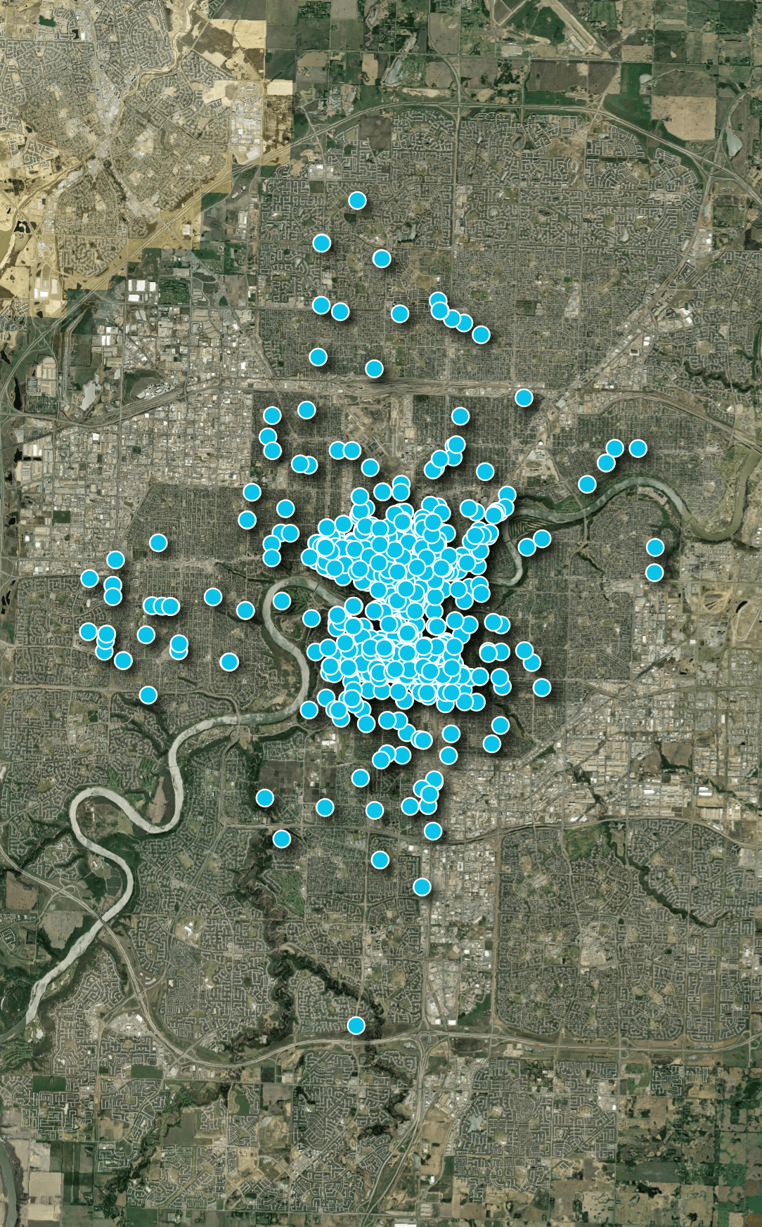
The first feed I'll analyse in this post is from Bird. Below are their bike locations across Edmonton as of Tuesday, May 5th, 2026 at 7AM. It was 0C at this time but it warmed to 10C by the afternoon.
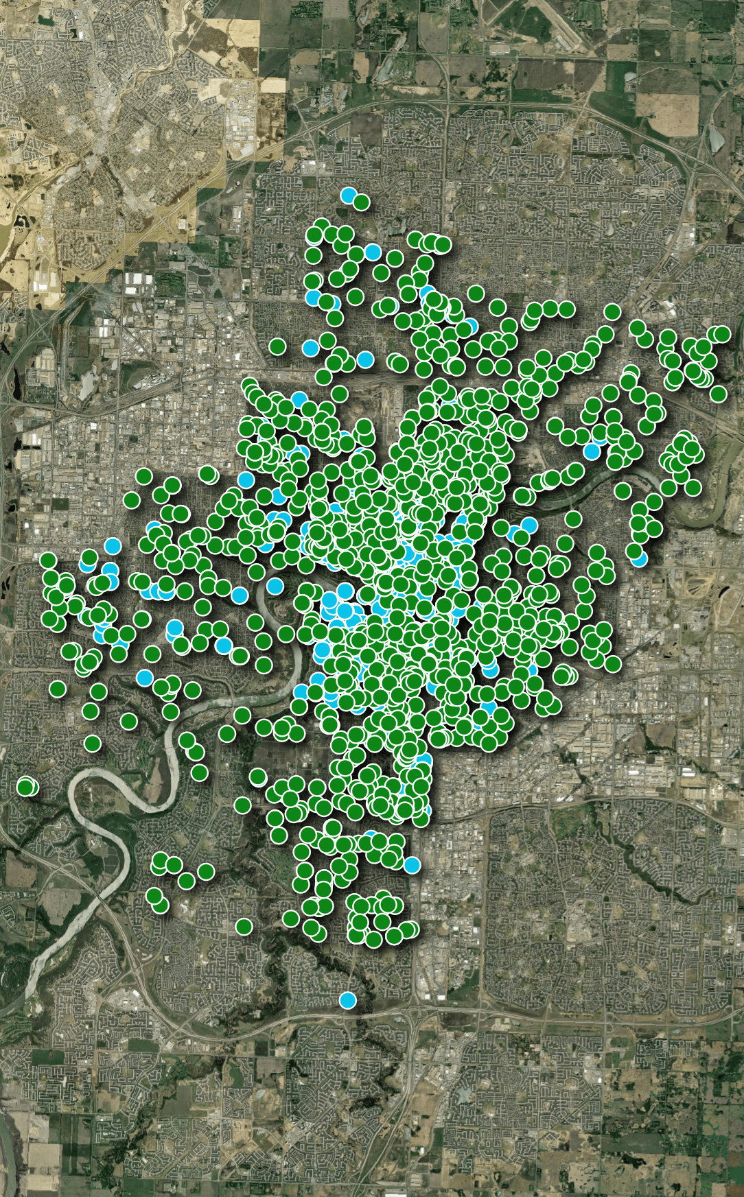
The second vendor is Lime. Below, their bike locations have been laid out in green on top of Bird's.
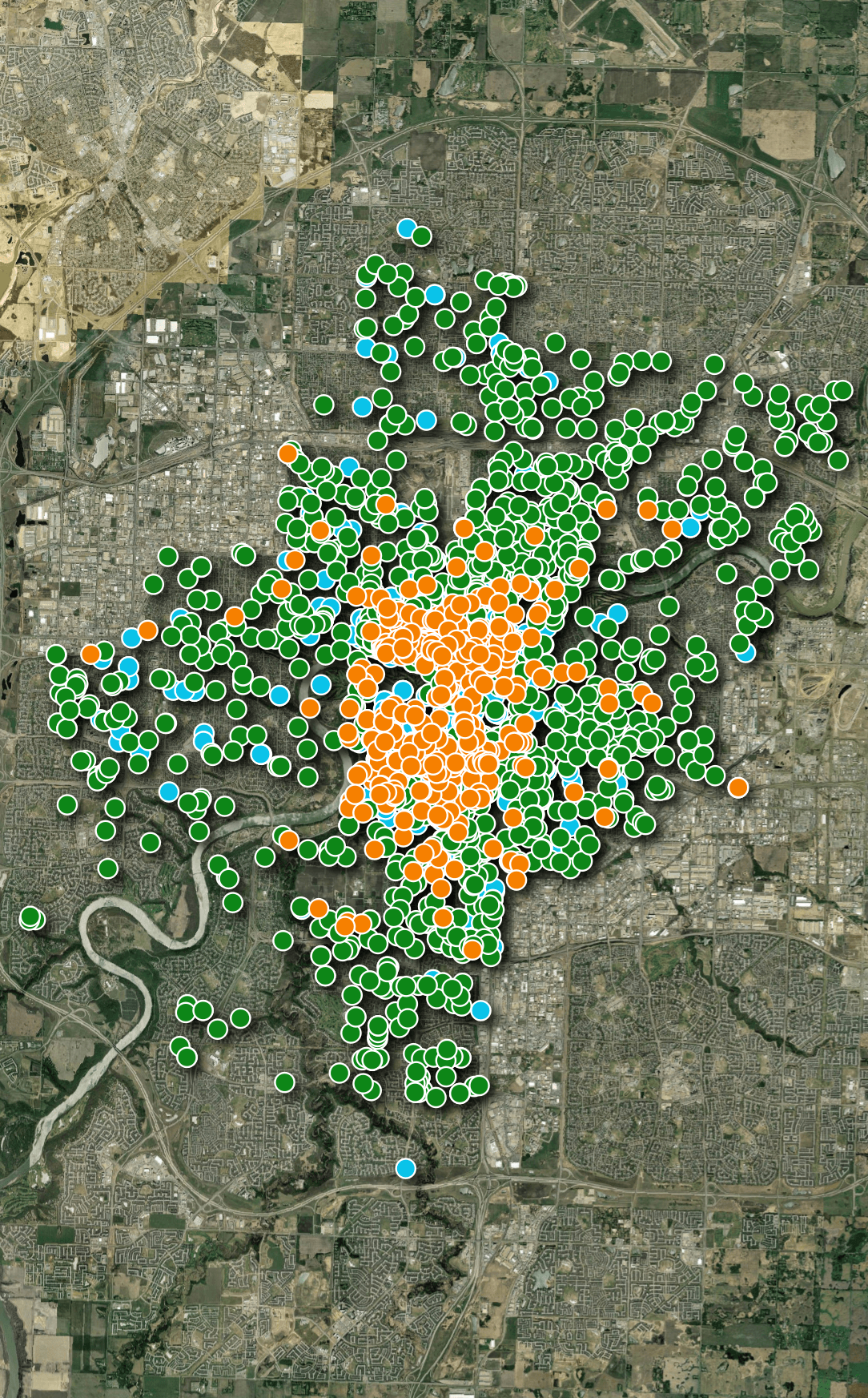
The third vendor is Neuron. Below, their bike locations have been laid out in orange on top of Bird's and Lime's.
Below is a heatmap showing which vendor has the most bikes in any one hexagon as of 7AM yesterday.
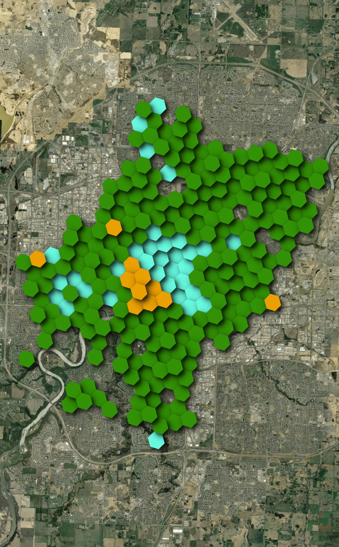
Fleet Snapshots
I collected JSON files from each of the three vendors for 12 of the 13 hours between 10AM and 10PM local time in Edmonton yesterday. The only gap was the 2PM download which failed for all three for some reason.
$ mkdir -p ~/ebikes_edmonton
$ cd ~/ebikes_edmonton

$ while :
  do
      DATE=`date --date="NOW" +"%Y.%m.%d.%H.%M.%S"`

      wget -O lime.$DATE.json   https://data.lime.bike/api/partners/v2/gbfs/edmonton/free_bike_status.json
      wget -O bird.$DATE.json   https://mds.bird.co/gbfs/v2/public/edmonton/free_bike_status.json
      wget -O neuron.$DATE.json https://mds.neuron-mobility.com/yeg/gbfs/2/en/free_bike_status

      echo "Sleeping for an hour.."
      sleep 3600
  done
Lime serves their responses via Cloudflare, Bird are from AWS Cloudfront and Neuron via Google Cloud.
The JSON filenames are prefixed with the name of the vendor, followed by the local time here in Estonia.
The JSON files are between 142 KB and 340 KB each.
Data Fluency
The feeds are very similar but do contain some differences. Neuron doesn't have a "last_reported" field but it's the only feed with a "station_id" field. This field was blank in every response I got from them. Below is an example record:
$ jq -S '.data.bikes[0]' \
    neuron.2026.05.06.11.22.20.json
{
  "bike_id": "e4c7de34-6c4b-3e7c-a147-c82dc07e12a5",
  "current_range_meters": 39500.0,
  "is_disabled": false,
  "is_reserved": false,
  "lat": 53.539043,
  "lon": -113.49915,
  "station_id": null,
  "vehicle_type_id": "e8fbc1f0-3504-3dff-852a-9e6dab5e204d"
}
Bird is the only feed with a "current_fuel_percent" field. Below is an example record.
$ jq -S '.data.bikes[0]' \
    bird.2026.05.05.19.55.10.json
{
  "bike_id": "c67cce09-ba6d-4114-86e2-0416f5d80ed4",
  "current_fuel_percent": 0.6363636,
  "current_range_meters": 21616.0,
  "is_disabled": false,
  "is_reserved": false,
  "last_reported": 1777999880,
  "lat": 53.5559835,
  "lon": -113.48228766666668,
  "vehicle_type_id": "bae2102b-56ba-42ba-9097-720e5990b4b2"
}
Lime has a textual "vehicle_type" field; the others use UUIDs. Below is an example record.
$ jq -S '.data.bikes[0]' \
    lime.2026.05.05.19.55.10.json
{
  "bike_id": "36a377ae-7bf9-42a9-902d-65efc0e99e9a",
  "current_range_meters": 38705,
  "is_disabled": false,
  "is_reserved": false,
  "last_reported": 1778000064,
  "lat": 53.522562,
  "lon": -113.51187,
  "vehicle_type": "scooter",
  "vehicle_type_id": "2"
}
Analysis-Ready Data
Below, I'll import each JSON file into vendor-specific tables in DuckDB.
$ touch bikes.duckdb; rm bikes.duckdb

$ for FILENAME in *.json; do
      VENDOR=`echo $FILENAME | cut -d. -f1`

      echo "CREATE OR REPLACE TABLE loading AS
              WITH a AS (
                  SELECT UNNEST(data.bikes) b
                  FROM   '$FILENAME'
              )
              SELECT b.*
              FROM   a;

            ALTER TABLE loading
            ADD COLUMN  source TEXT;

            UPDATE loading
            SET    source = '$FILENAME';

            CREATE TABLE IF NOT EXISTS $VENDOR AS
              FROM  loading
              LIMIT 0;

            INSERT INTO $VENDOR
            FROM        loading;

            DROP TABLE loading;
            " | ~/duckdb bikes.duckdb
  done
I'll merge the compatible fields from all three vendor tables into a single "bikes" table.
$ ~/duckdb bikes.duckdb
CREATE OR REPLACE TABLE bikes AS
    SELECT vendor: 'Bird',
           bike_id,
           geometry: ST_POINT(lon, lat),
           is_disabled,
           is_reserved,
           vehicle_type_id: vehicle_type_id::TEXT,
           vehicle_type: 'Unknown',
           current_range_meters,
           source,
           downloaded_at:
            MAKE_TIMESTAMPTZ(
                SPLIT(source, '.')[2]::BIGINT,
                SPLIT(source, '.')[3]::BIGINT,
                SPLIT(source, '.')[4]::BIGINT,
                SPLIT(source, '.')[5]::BIGINT,
                SPLIT(source, '.')[6]::BIGINT,
                SPLIT(source, '.')[7]::BIGINT,
                'Europe/Tallinn')
    FROM bird

    UNION ALL BY NAME

    SELECT vendor: 'Lime',
           bike_id,
           geometry: ST_POINT(lon, lat),
           is_disabled,
           is_reserved,
           vehicle_type_id: vehicle_type_id::TEXT,
           vehicle_type,
           current_range_meters,
           source,
           downloaded_at:
            MAKE_TIMESTAMPTZ(
                SPLIT(source, '.')[2]::BIGINT,
                SPLIT(source, '.')[3]::BIGINT,
                SPLIT(source, '.')[4]::BIGINT,
                SPLIT(source, '.')[5]::BIGINT,
                SPLIT(source, '.')[6]::BIGINT,
                SPLIT(source, '.')[7]::BIGINT,
                'Europe/Tallinn')
    FROM lime

    UNION ALL BY NAME

    SELECT vendor: 'Neuron',
           bike_id,
           geometry: ST_POINT(lon, lat),
           is_disabled,
           is_reserved,
           vehicle_type_id: vehicle_type_id::TEXT,
           vehicle_type: 'Unknown',
           current_range_meters,
           source,
           downloaded_at:
            MAKE_TIMESTAMPTZ(
                SPLIT(source, '.')[2]::BIGINT,
                SPLIT(source, '.')[3]::BIGINT,
                SPLIT(source, '.')[4]::BIGINT,
                SPLIT(source, '.')[5]::BIGINT,
                SPLIT(source, '.')[6]::BIGINT,
                SPLIT(source, '.')[7]::BIGINT,
                'Europe/Tallinn')
    FROM neuron;
The above produced a 50,972-row, 10-column table. The following is an example record.
$ echo "FROM  bikes
        LIMIT 1" \
    | ~/duckdb -json bikes.duckdb \
    | jq -S .
[
  {
    "bike_id": "c67cce09-ba6d-4114-86e2-0416f5d80ed4",
    "current_range_meters": 21616.0,
    "downloaded_at": "2026-05-05 19:55:10+03",
    "geometry": "POINT (-113.48228766666668 53.5559835)",
    "is_disabled": "false",
    "is_reserved": "false",
    "source": "bird.2026.05.05.19.55.10.json",
    "vehicle_type": "Unknown",
    "vehicle_type_id": "bae2102b-56ba-42ba-9097-720e5990b4b2",
    "vendor": "Bird"
  }
]
e-Bike Availability
Below, I'll count the number of unique bike IDs per vendor per hour. The timestamp field is the local time in Edmonton.
$ ~/duckdb bikes.duckdb
WITH a AS (
    SELECT   date_hour: (TIMEZONE('Canada/Mountain', downloaded_at)::DATE || ' ' ||
                         HOUR(TIMEZONE('Canada/Mountain', downloaded_at)) || ':00:00')::TIMESTAMP,
             vendor,
             num_recs:  COUNT(DISTINCT bike_id)
    FROM     bikes
    GROUP BY 1, 2
)
PIVOT    a
ON       vendor
USING    SUM(num_recs)
GROUP BY date_hour
ORDER BY date_hour;
┌─────────────────────┬────────┬────────┬────────┐
│      date_hour      │  Bird  │  Lime  │ Neuron │
│      timestamp      │ int128 │ int128 │ int128 │
├─────────────────────┼────────┼────────┼────────┤
│ 2026-05-05 10:00:00 │   1110 │   1409 │    626 │
│ 2026-05-05 11:00:00 │   1127 │   1395 │    637 │
│ 2026-05-05 12:00:00 │   1153 │   1392 │    637 │
│ 2026-05-05 13:00:00 │   1149 │   1386 │    645 │
│ 2026-05-05 15:00:00 │   1153 │   1392 │    651 │
│ 2026-05-05 16:00:00 │   1157 │   1354 │    647 │
│ 2026-05-05 17:00:00 │   1196 │   1359 │    634 │
│ 2026-05-05 18:00:00 │   1215 │   1368 │    633 │
│ 2026-05-05 19:00:00 │   1205 │   1380 │    641 │
│ 2026-05-05 20:00:00 │   1195 │   1366 │    636 │
│ 2026-05-05 21:00:00 │   1208 │   1394 │    643 │
│ 2026-05-05 22:00:00 │   1222 │   1410 │    650 │
└─────────────────────┴────────┴────────┴────────┘
Rotating Bike IDs
Judging by the unique bike ID counts, Bird and Lime appear to rotate the IDs for their bikes at least every hour. Neuron appears to only use one ID per bike over the period I was observing their feed.
$ ~/duckdb bikes.duckdb
SELECT   vendor,
         num_bikes: COUNT(DISTINCT bike_id)
FROM     bikes
GROUP BY 1;
┌─────────┬───────────┐
│ vendor  │ num_bikes │
│ varchar │   int64   │
├─────────┼───────────┤
│ Bird    │     14090 │
│ Lime    │     16605 │
│ Neuron  │       657 │
└─────────┴───────────┘
Bike Types
Each vendor has two types of bikes on offer in Edmonton. Below are their type identifiers.
$ ~/duckdb bikes.duckdb
SELECT   DISTINCT vendor,
                  vehicle_type,
                  vehicle_type_id
FROM     bikes
GROUP BY 1, 2, 3
ORDER BY 1;
┌─────────┬──────────────┬──────────────────────────────────────┐
│ vendor  │ vehicle_type │           vehicle_type_id            │
│ varchar │   varchar    │               varchar                │
├─────────┼──────────────┼──────────────────────────────────────┤
│ Bird    │ Unknown      │ bae2102b-56ba-42ba-9097-720e5990b4b2 │
│ Bird    │ Unknown      │ 2ea3c8b2-ed07-4c53-b87e-638c08471309 │
│ Lime    │ e-bike       │ 3                                    │
│ Lime    │ scooter      │ 2                                    │
│ Neuron  │ Unknown      │ 9e8e37ae-b444-3d57-9e9a-58ce02e9f2fd │
│ Neuron  │ Unknown      │ e8fbc1f0-3504-3dff-852a-9e6dab5e204d │
└─────────┴──────────────┴──────────────────────────────────────┘
There aren't a lot of bike capabilities listed within the feeds I monitored. I searched for "bae2102b-56ba-42ba-9097-720e5990b4b2" which brought up this Japanese-language site with the following JSON snippet for two of Bird's bikes:
[
    {
        "vehicle_type_id": "bae2102b-56ba-42ba-9097-720e5990b4b2",
        "form_factor": "scooter",
        "propulsion_type": "electric",
        "max_range_meters": 24000
    },
    {
        "vehicle_type_id": "2ea3c8b2-ed07-4c53-b87e-638c08471309",
        "form_factor": "bicycle",
        "propulsion_type": "electric_assist",
        "max_range_meters": 60000
    }
]
There is further work to collect the metadata around each vendor's fleet capabilities as it could uncover some interesting trends.
Bike Ranges
Below are the number of bikes available, binned by their range and rounded up to the nearest 10 KM. Lime was the only vendor with 60KM+ bikes available at the time of this observation.
$ ~/duckdb bikes.duckdb
WITH a AS (
    SELECT   range_km: (current_range_meters/10000)::INT*10,
             vendor,
             num_recs: COUNT(DISTINCT bike_id)
    FROM     bikes
    WHERE    downloaded_at::TEXT LIKE '2026-05-05 20%'
    GROUP BY 1, 2
)
PIVOT    a
ON       vendor
USING    SUM(num_recs)
GROUP BY range_km
ORDER BY range_km;
┌──────────┬────────┬────────┬────────┐
│ range_km │  Bird  │  Lime  │ Neuron │
│  int32   │ int128 │ int128 │ int128 │
├──────────┼────────┼────────┼────────┤
│        0 │     12 │    125 │     21 │
│       10 │    286 │    284 │     65 │
│       20 │    358 │    227 │    149 │
│       30 │    383 │    257 │    146 │
│       40 │     86 │    329 │    121 │
│       50 │      2 │     45 │    135 │
│       60 │   NULL │     69 │   NULL │
│       70 │   NULL │     57 │   NULL │
│       80 │   NULL │      2 │   NULL │
└──────────┴────────┴────────┴────────┘
Bike Footprints
Below, I'll calculate each Neuron's bikes' bounding box for all of its journeys over the day I monitored their feed. Note, I only have snapshots of their location every hour and a bike will only show up if it's available so there is room for error in these measurements.
$ ~/duckdb bikes.duckdb
CREATE OR REPLACE TABLE neuron_extents AS
    WITH a AS (
        SELECT   bike_id,
                 geometry: {'min_x': MIN(ST_X(ST_CENTROID(geometry))),
                            'min_y': MIN(ST_Y(ST_CENTROID(geometry))),
                            'max_x': MAX(ST_X(ST_CENTROID(geometry))),
                            'max_y': MAX(ST_Y(ST_CENTROID(geometry)))}::BOX_2D::GEOMETRY,
        FROM     bikes
        WHERE    vendor = 'Neuron'
        GROUP BY 1
        ORDER BY 2 DESC
    )
    SELECT bike_id,
           area_size: ST_AREA(geometry)
    FROM   a;
Of Neuron's 657 bikes, only 76 hadn't moved at all throughout the day.
SELECT   no_movement: area_size=0.0,
         COUNT(*)
FROM     neuron_extents
GROUP BY 1;
┌─────────────┬──────────────┐
│ no_movement │ count_star() │
│   boolean   │    int64     │
├─────────────┼──────────────┤
│ false       │          581 │
│ true        │           76 │
└─────────────┴──────────────┘
I'll build a trajectory map of their 20 most-travelled bikes for the period I was observing their feed.
COPY (
   SELECT   * EXCLUDE (geometry, bike_id),
            bike_id:  bike_id::TEXT,
            bbox:     {'xmin': ST_XMIN(ST_EXTENT(geometry)),
                       'ymin': ST_YMIN(ST_EXTENT(geometry)),
                       'xmax': ST_XMAX(ST_EXTENT(geometry)),
                       'ymax': ST_YMAX(ST_EXTENT(geometry))},
            geometry: ST_ASWKB(geometry)
   FROM     bikes
   WHERE    bike_id IN (
                SELECT   bike_id
                FROM     neuron_extents
                ORDER BY area_size DESC
                LIMIT    20)
   ORDER BY HILBERT_ENCODE([ST_Y(ST_CENTROID(geometry)),
                            ST_X(ST_CENTROID(geometry))]::double[2])
) TO 'Neuron.parquet' (
   FORMAT            'PARQUET',
   CODEC             'ZSTD',
   COMPRESSION_LEVEL 22,
   ROW_GROUP_SIZE    15000);
The maps in the screenshots below are projected with EPSG:3771. After adding any Parquet file into QGIS, select its layer properties and then under source, change its assigned coordinate system (CRS) to EPSG:4326.
I'll search for and select "Create trajectories" in the Processing Toolbox.
I've set the input point layer to the "Neuron" one that contains the data from the Parquet file I generated above. I've also set the Trajectory ID field to "bike_id" and the timestamp field to "downloaded_at".
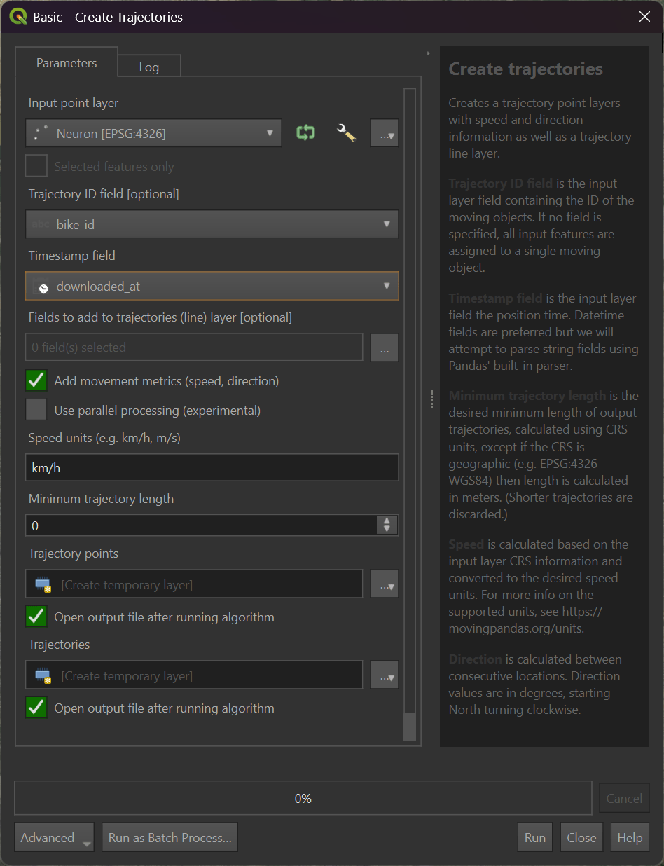
After hitting run, the following was generated. The extent of the map is ~11.4 KM tall by ~7 KM wide. The start of each bike's journey is in blue and follows a gradient till they reach red at the end.
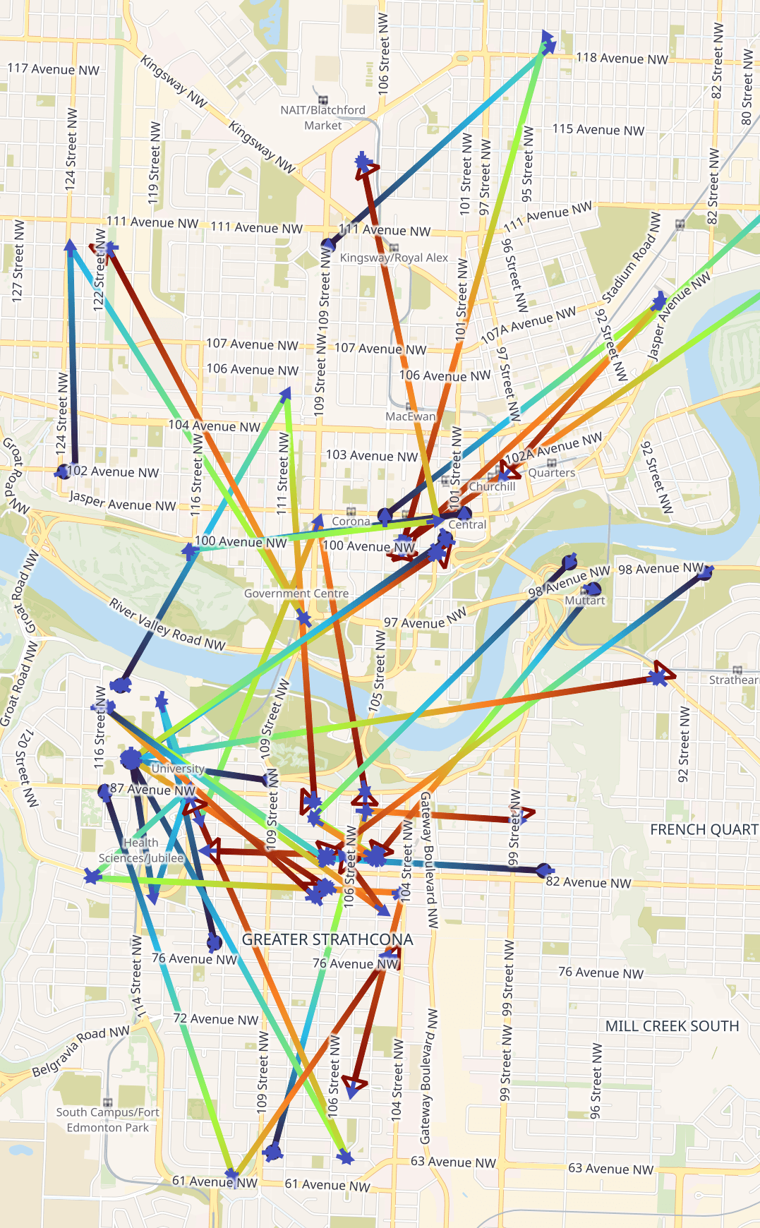
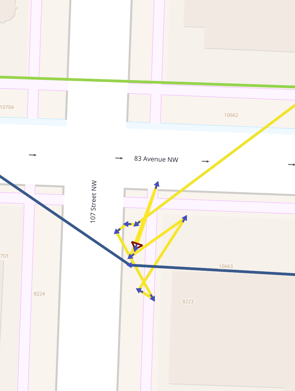
I did notice that some bikes moved short distances hour-by-hour during certain time windows. This could be down to GPS drift or people moving the bike out of the way.
Trajectools supports loitering analysis which could go some way to determine how many Neuron bikes made significant journeys. Below I'll export all of Neuron's journeys to a Parquet file.
$ ~/duckdb bikes.duckdb
COPY (
   SELECT   * EXCLUDE (geometry, bike_id),
            bike_id:  bike_id::TEXT,
            bbox:     {'xmin': ST_XMIN(ST_EXTENT(geometry)),
                       'ymin': ST_YMIN(ST_EXTENT(geometry)),
                       'xmax': ST_XMAX(ST_EXTENT(geometry)),
                       'ymax': ST_YMAX(ST_EXTENT(geometry))},
            geometry: ST_ASWKB(geometry)
   FROM     bikes
   WHERE    vendor = 'Neuron'
   ORDER BY HILBERT_ENCODE([ST_Y(ST_CENTROID(geometry)),
                            ST_X(ST_CENTROID(geometry))]::double[2])
) TO 'Neuron.all_day.parquet' (
   FORMAT            'PARQUET',
   CODEC             'ZSTD',
   COMPRESSION_LEVEL 22,
   ROW_GROUP_SIZE    15000);
I've imported that into QGIS and run Trajectools' "Split trajectories at stops" tool with the following parameters.
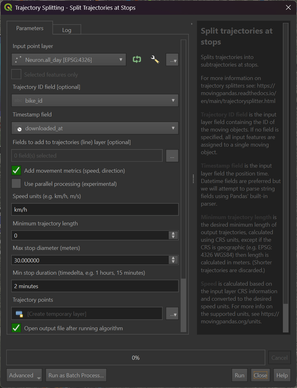
I exported a GeoPackage (GPKG) file of the resulting analysis. It appears only 160 Neuron bikes moved more than 1 KM throughout the day.
$ ~/duckdb bikes.duckdb
SELECT num_bikes: COUNT(DISTINCT(bike_id))
FROM   ST_READ('Neuron.traj.gpkg')
WHERE  length_km > 1;
┌───────────┐
│ num_bikes │
│   int64   │
├───────────┤
│       160 │
└───────────┘
Changing Availability
Below, I'll generate a heatmap of the number of bikes available across all vendors throughout the day I observed their feeds.
$ ~/duckdb bikes.duckdb
CREATE OR REPLACE TABLE h3_stats AS
    SELECT   date_hour: (TIMEZONE('Canada/Mountain', downloaded_at)::DATE || ' ' ||
                         HOUR(TIMEZONE('Canada/Mountain', downloaded_at)) || ':00:00')::TIMESTAMP,
             hexagon:   H3_LATLNG_TO_CELL(
                          ST_Y(ST_CENTROID(geometry)),
                          ST_X(ST_CENTROID(geometry)),
                          7),
             num_recs:  COUNT(DISTINCT bike_id)
    FROM     bikes
    GROUP BY 1, 2;

COPY (
    SELECT geometry: ST_ASWKB(H3_CELL_TO_BOUNDARY_WKT(hexagon)::geometry),
           date_hour,
           num_recs
    FROM   h3_stats
) TO 'bikes_per_hour.h3_4.parquet' (
        FORMAT 'PARQUET',
        CODEC  'ZSTD',
        COMPRESSION_LEVEL 22,
        ROW_GROUP_SIZE 15000);
Regardless of the time of day, there is a fairly consistent availability in just about every hexagon.