Data Crew is a consultancy that was started last year in Argentina. They've recently released a 1,419-line, Python-based Route Optimiser Framework.
It supports both the Chinese Postman (CPP) and Travelling Salesman (TSP) problems. The framework is meant to be easy to expand and there are plans to add support for Vehicle Routing (VRP), Capacitated VRP (CVRP) and VRP with Time Windows (VRPTW) at a later date.
In this post, I'll examine two example solvers from Data Crew's Route Optimiser Framework.
My Workstation
I'm using a 5.7 GHz AMD Ryzen 9 9950X CPU. It has 16 cores and 32 threads and 1.2 MB of L1, 16 MB of L2 and 64 MB of L3 cache. It has a liquid cooler attached and is housed in a spacious, full-sized Cooler Master HAF 700 computer case.
The system has 96 GB of DDR5 RAM clocked at 4,800 MT/s and a 5th-generation, Crucial T700 4 TB NVMe M.2 SSD which can read at speeds up to 12,400 MB/s. There is a heatsink on the SSD to help keep its temperature down. This is my system's C drive.
The system is powered by a 1,200-watt, fully modular Corsair Power Supply and is sat on an ASRock X870E Nova 90 Motherboard.
I'm running Ubuntu 24 LTS via Microsoft's Ubuntu for Windows on Windows 11 Pro. In case you're wondering why I don't run a Linux-based desktop as my primary work environment, I'm still using an Nvidia GTX 1080 GPU which has better driver support on Windows and ArcGIS Pro only supports Windows natively.
Installing Prerequisites
I'll use Python 3.12.3 and jq to help analyse the data in this post.
$ sudo add-apt-repository ppa:deadsnakes/ppa
$ sudo apt update
$ sudo apt install \
    jq \
    python3-pip \
    python3.12-venv
Below, I'll set up a Python Virtual Environment and install some dependencies.
$ python3 -m venv ~/.route-optimizer
$ source ~/.route-optimizer/bin/activate
$ python3 -m pip install \
    contextily \
    folium \
    geopandas \
    matplotlib \
    networkx \
    openpyxl \
    osmnx \
    pandas \
    scikit-learn \
    shapely
I'll clone the repo that contains the framework as well as some example scenarios that I'll walk through below.
$ git clone https://github.com/Data-Crew/route-optimizer \
    ~/route-optimizer
I'll use DuckDB v1.4.3, along with its H3, JSON, Lindel, Parquet and Spatial extensions, in this post.
$ cd ~
$ wget -c https://github.com/duckdb/duckdb/releases/download/v1.4.3/duckdb_cli-linux-amd64.zip
$ unzip -j duckdb_cli-linux-amd64.zip
$ chmod +x duckdb
$ ~/duckdb
INSTALL h3 FROM community;
INSTALL lindel FROM community;
INSTALL json;
INSTALL parquet;
INSTALL spatial;
I'll set up DuckDB to load every installed extension each time it launches.
$ vi ~/.duckdbrc
.timer on
.width 180
LOAD h3;
LOAD lindel;
LOAD json;
LOAD parquet;
LOAD spatial;
Parking Enforcement
The first example is a parking enforcement solver. An inspector needs the shortest path along a circuit that visits every edge at least once.
Below is the configuration file that this solver will call upon. It isolates a bounding box around La Plata, Argentina, a planned city with diagonal avenues, which is to the southeast of Buenos Aires.
This bounding box will be used to isolate the OpenStreetMap (OSM) road network for this area via the OSMnx library.
There are also three zones defined within this area, each with its own unique parking restrictions.
$ cd ~/route-optimizer
$ cat zone_config.json
{
  "configuration": {
    "city": "La Plata, Argentina",
    "bbox": {
      "description": "Bounding box (west, south, east, north)",
      "west": -57.9605,
      "south": -34.9210,
      "east": -57.9455,
      "north": -34.9095
    },
    "start_point": {
      "description": "Start and return point (lat, lon)",
      "name": "Corner of 12th and 50th",
      "latitude": -34.91719,
      "longitude": -57.95067
    }
  },
  "zones": [
    {
      "name": "courthouse",
      "description": "Courthouse Zone",
      "polygon": [
        [-57.957, -34.915],
        [-57.949, -34.915],
        [-57.949, -34.911],
        [-57.957, -34.911]
      ],
      "schedule": {
        "start": "08:00",
        "end": "14:00"
      },
      "weekdays": [0, 1, 2, 3, 4],
      "weekday_names": ["Monday", "Tuesday", "Wednesday", "Thursday", "Friday"],
      "prohibited_streets": [],
      "color": "pink"
    },
    {
      "name": "downtown",
      "description": "Downtown Zone",
      "polygon": [
        [-57.955, -34.9145],
        [-57.9475, -34.9145],
        [-57.9475, -34.9185],
        [-57.955, -34.9185]
      ],
      "schedule": {
        "start": "08:00",
        "end": "20:00"
      },
      "weekdays": [0, 1, 2, 3, 4, 5],
      "weekday_names": ["Monday", "Tuesday", "Wednesday", "Thursday", "Friday", "Saturday"],
      "prohibited_streets": [],
      "color": "gold"
    },
    {
      "name": "12th_street",
      "description": "12th Street Zone",
      "polygon": [
        [-57.955, -34.9125],
        [-57.952, -34.9125],
        [-57.952, -34.9195],
        [-57.955, -34.9195]
      ],
      "schedule": {
        "start": "08:00",
        "end": "20:00"
      },
      "weekdays": [0, 1, 2, 3, 4, 5],
      "weekday_names": ["Monday", "Tuesday", "Wednesday", "Thursday", "Friday", "Saturday"],
      "prohibited_streets": [],
      "color": "violet"
    }
  ],
  "route_types": {
    "full": {
      "name": "Full Route",
      "description": "All zones (Monday to Friday 8am-8pm)",
      "zones": ["courthouse", "downtown", "12th_street"]
    },
    "no_courthouse": {
      "name": "No Courthouse",
      "description": "For enforcement officers working after 2pm",
      "zones": ["downtown", "12th_street"]
    },
    "saturday": {
      "name": "Saturday",
      "description": "Weekend route",
      "zones": ["downtown", "12th_street"]
    }
  }
}
Below, I'll run the solver. This first deliverable is a map of the zone within the bounding box.
$ python3 parking_enforcement.py
======================================================================
 ROUTE OPTIMIZER - PARKING ENFORCEMENT (CPP)
======================================================================
📥 Downloading street network...
✅ Network downloaded: 208 nodes, 369 edges
📍 Start node: 249417335

🏷️  Labeling zones...
   • courthouse: 39 nodes
   • downtown: 34 nodes
   • 12th_street: 27 nodes

📊 Zone summary:
zone
outside        135
courthouse      29
12th_street     27
downtown        17
Name: count, dtype: int64

🗺️  Generating visualization...
💾 Map saved to: output/cpp_zones.png
Then, the full route is calculated and results in a solution that is 11.06 KM long.
======================================================================
 CALCULATING OPTIMAL ROUTES
======================================================================

📍 CASE 1: Full Route

============================================================
🚀 SOLVING ROUTE: FULL (CPP)
============================================================

🔍 Route type 'full':
   • Zones: courthouse, downtown, 12th_street
   • Nodes: 73
   • Edges: 123

🔄 Solving Chinese Postman Problem (CPP)...
   ⚠️  Graph not strongly connected. Extracting main component...
   🔄 Eulerizing graph...
      • 13 unbalanced nodes
      ✅ Eulerized: 139 edges
   🔍 Finding Eulerian circuit...
   ⚠️  Could not create perfect Eulerian circuit
   📍 Using approximation...
      📍 Expanded 11 path segments with intermediate nodes
   ✅ Route found: 119 nodes, 11.09 km

✅ Route calculated (CPP):
   • Nodes visited: 119
   • Total distance: 11.09 km
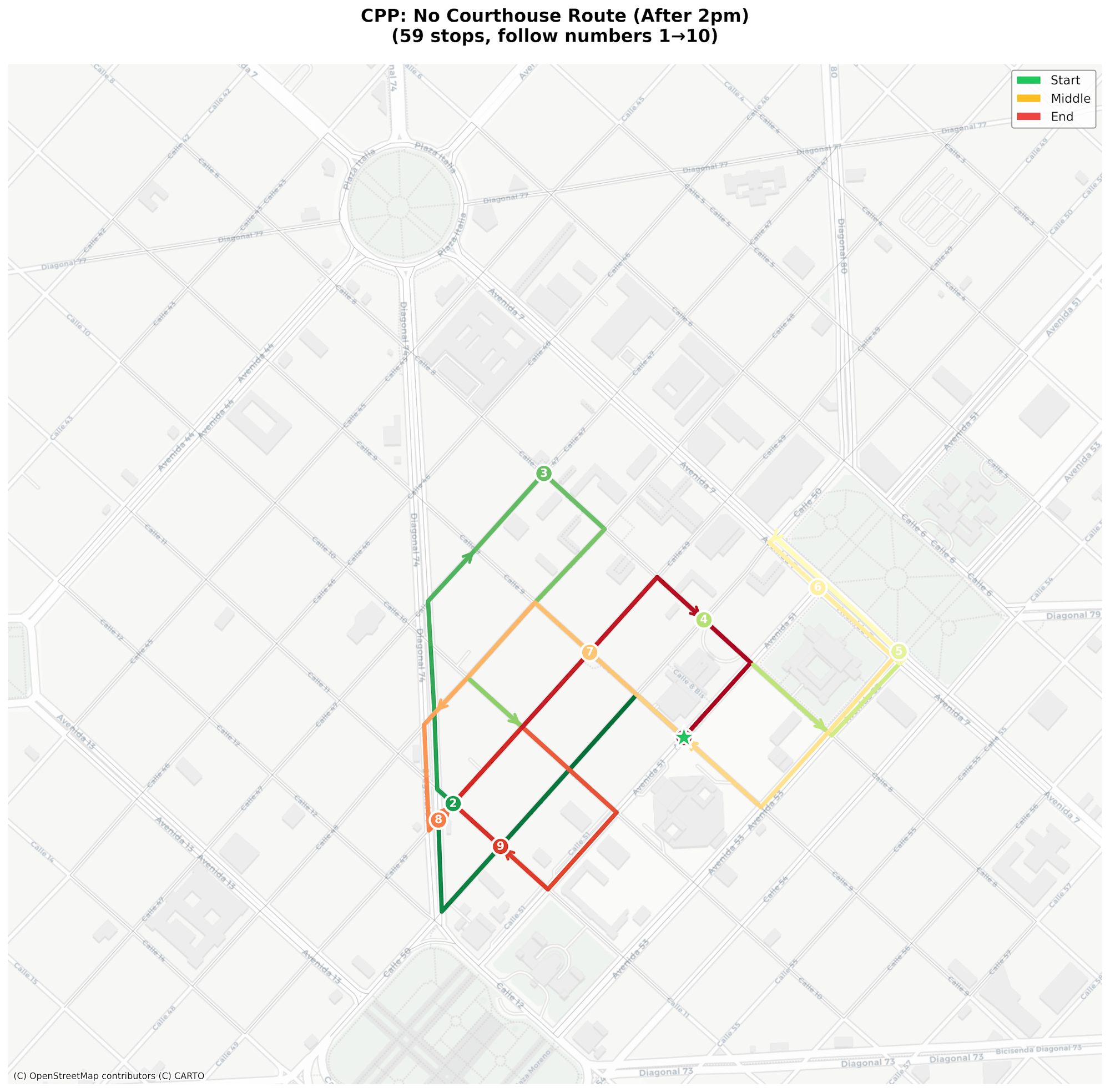
The next calculation handles the "no courthouse" custom restrictions and produces a solution with a distance of 5.39 KM.
📍 CASE 2: No Courthouse (after 2pm)

============================================================
🚀 SOLVING ROUTE: NO_COURTHOUSE (CPP)
============================================================

🔍 Route type 'no_courthouse':
   • Zones: downtown, 12th_street
   • Nodes: 44
   • Edges: 69

🔄 Solving Chinese Postman Problem (CPP)...
   ⚠️  Graph not strongly connected. Extracting main component...
   🔄 Eulerizing graph...
      • 10 unbalanced nodes
      ✅ Eulerized: 79 edges
   🔍 Finding Eulerian circuit...
   ⚠️  Could not create perfect Eulerian circuit
   📍 Using approximation...
      📍 Expanded 4 path segments with intermediate nodes
   ✅ Route found: 59 nodes, 5.39 km

✅ Route calculated (CPP):
   • Nodes visited: 59
   • Total distance: 5.39 km
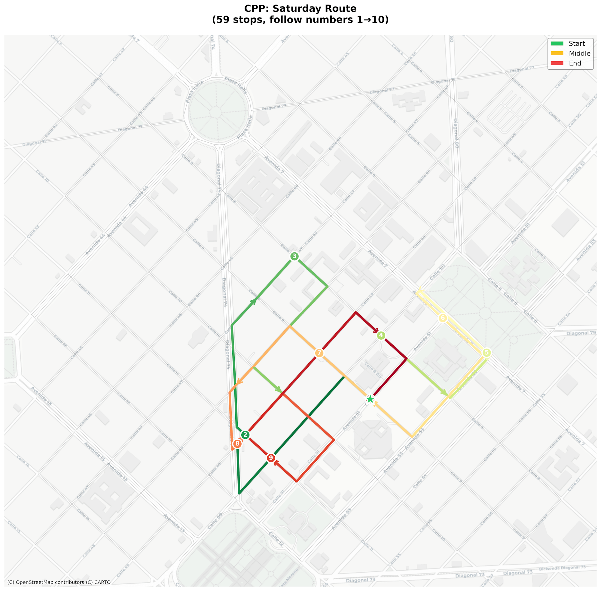
The next calculation handles the Saturday route and produces a solution with a distance of 5.39 KM.
📍 CASE 3: Saturday Route

============================================================
🚀 SOLVING ROUTE: SATURDAY (CPP)
============================================================

🔍 Route type 'saturday':
   • Zones: downtown, 12th_street
   • Nodes: 44
   • Edges: 69

🔄 Solving Chinese Postman Problem (CPP)...
   ⚠️  Graph not strongly connected. Extracting main component...
   🔄 Eulerizing graph...
      • 10 unbalanced nodes
      ✅ Eulerized: 79 edges
   🔍 Finding Eulerian circuit...
   ⚠️  Could not create perfect Eulerian circuit
   📍 Using approximation...
      📍 Expanded 4 path segments with intermediate nodes
   ✅ Route found: 59 nodes, 5.39 km

✅ Route calculated (CPP):
   • Nodes visited: 59
   • Total distance: 5.39 km
The results of the three above cases are then saved to an Excel file.
📊 Exporting results...
✅ Results exported to: output/cpp_routes.xlsx

📋 Summary:
   Route_Type  Node_Count  Distance_KM  Distance_Meters
         full         119        11.09            11093
no_courthouse          59         5.39             5392
     saturday          59         5.39             5392
Below is the summary sheet from that file.
$ echo "FROM ST_READ('output/cpp_routes.xlsx')" \
    | ~/duckdb -json \
    | jq -S .
[
  {
    "Distance_KM": 11.09,
    "Distance_Meters": 11093,
    "Node_Count": 119,
    "Route_Type": "full"
  },
  {
    "Distance_KM": 5.39,
    "Distance_Meters": 5392,
    "Node_Count": 59,
    "Route_Type": "no_courthouse"
  },
  {
    "Distance_KM": 5.39,
    "Distance_Meters": 5392,
    "Node_Count": 59,
    "Route_Type": "saturday"
  }
]
Each case has its own sheet with its sequence list. Below is the sheet for the Saturday route.
$ ~/duckdb
.maxrows 60

SELECT sequence: Sequence::INT,
       node_id:  Node_ID::BIGINT,
       geom:     ST_POINT(Longitude, Latitude),
       zone:     Zone
FROM   READ_XLSX('output/cpp_routes.xlsx',
                 sheet='saturday');
┌──────────┬────────────┬─────────────────────────────────┬─────────────┐
│ sequence │  node_id   │              geom               │    zone     │
│  int32   │   int64    │            geometry             │   varchar   │
├──────────┼────────────┼─────────────────────────────────┼─────────────┤
│        1 │  249417335 │ POINT (-57.9510606 -34.91725)   │ downtown    │
│        2 │  249417330 │ POINT (-57.9517689 -34.9167244) │ downtown    │
│        3 │  249417040 │ POINT (-57.9527766 -34.9176466) │ 12th_street │
│        4 │  249416478 │ POINT (-57.9538079 -34.9185892) │ 12th_street │
│        5 │ 6127585995 │ POINT (-57.9546872 -34.9193893) │ 12th_street │
│        6 │ 6127586000 │ POINT (-57.9547393 -34.918265)  │ 12th_street │
│        7 │  249416467 │ POINT (-57.9545168 -34.9180625) │ 12th_street │
│        8 │  249416459 │ POINT (-57.9547554 -34.9178853) │ 12th_street │
│        9 │  249418061 │ POINT (-57.954798 -34.9169539)  │ 12th_street │
│       10 │  249417004 │ POINT (-57.9548565 -34.9161046) │ 12th_street │
│       11 │  249418057 │ POINT (-57.9548928 -34.9155776) │ 12th_street │
│       12 │  249417305 │ POINT (-57.9541766 -34.9149376) │ 12th_street │
│       13 │  249417664 │ POINT (-57.9531609 -34.9140082) │ 12th_street │
│       14 │  249417665 │ POINT (-57.9522478 -34.9146926) │ 12th_street │
│       15 │  249417312 │ POINT (-57.9532914 -34.9155946) │ 12th_street │
│       16 │  249417026 │ POINT (-57.9543003 -34.9165164) │ 12th_street │
│       17 │  249417033 │ POINT (-57.9534809 -34.9171231) │ 12th_street │
│       18 │  249417320 │ POINT (-57.9524713 -34.9162031) │ 12th_street │
│       19 │  249417672 │ POINT (-57.9514609 -34.9152824) │ downtown    │
│       20 │  249417675 │ POINT (-57.9507639 -34.9158047) │ downtown    │
│       21 │  249417679 │ POINT (-57.9500587 -34.9163333) │ downtown    │
│       22 │ 1868768411 │ POINT (-57.948899 -34.9171887)  │ downtown    │
│       23 │  249417681 │ POINT (-57.9488464 -34.9172257) │ downtown    │
│       24 │ 2761285280 │ POINT (-57.9478281 -34.9163417) │ downtown    │
│       25 │ 1868768407 │ POINT (-57.9477386 -34.9162624) │ downtown    │
│       26 │ 2714068787 │ POINT (-57.9478392 -34.9161947) │ downtown    │
│       27 │ 2761285279 │ POINT (-57.9479159 -34.9162708) │ downtown    │
│       28 │ 2761285280 │ POINT (-57.9478281 -34.9163417) │ downtown    │
│       29 │ 1868768407 │ POINT (-57.9477386 -34.9162624) │ downtown    │
│       30 │ 2714068787 │ POINT (-57.9478392 -34.9161947) │ downtown    │
│       31 │  249417867 │ POINT (-57.9496921 -34.9147895) │ downtown    │
│       32 │ 2761285275 │ POINT (-57.949781 -34.9148569)  │ downtown    │
│       33 │ 2761285277 │ POINT (-57.9490549 -34.9154107) │ downtown    │
│       34 │ 2761285279 │ POINT (-57.9479159 -34.9162708) │ downtown    │
│       35 │ 1868768411 │ POINT (-57.948899 -34.9171887)  │ downtown    │
│       36 │ 1868768422 │ POINT (-57.9499061 -34.9181067) │ downtown    │
│       37 │  249417335 │ POINT (-57.9510606 -34.91725)   │ downtown    │
│       38 │  249417330 │ POINT (-57.9517689 -34.9167244) │ downtown    │
│       39 │  249417320 │ POINT (-57.9524713 -34.9162031) │ 12th_street │
│       40 │  249417312 │ POINT (-57.9532914 -34.9155946) │ 12th_street │
│       41 │  249417026 │ POINT (-57.9543003 -34.9165164) │ 12th_street │
│       42 │  249418061 │ POINT (-57.954798 -34.9169539)  │ 12th_street │
│       43 │ 6127586001 │ POINT (-57.954951 -34.9170952)  │ 12th_street │
│       44 │ 6127585996 │ POINT (-57.9549152 -34.9177665) │ 12th_street │
│       45 │ 2760842529 │ POINT (-57.9548801 -34.9183932) │ 12th_street │
│       46 │ 6127586000 │ POINT (-57.9547393 -34.918265)  │ 12th_street │
│       47 │  249416467 │ POINT (-57.9545168 -34.9180625) │ 12th_street │
│       48 │  249417033 │ POINT (-57.9534809 -34.9171231) │ 12th_street │
│       49 │  249417040 │ POINT (-57.9527766 -34.9176466) │ 12th_street │
│       50 │  249417046 │ POINT (-57.9520687 -34.9181727) │ 12th_street │
│       51 │  249416487 │ POINT (-57.9530977 -34.9191169) │ 12th_street │
│       52 │  249416478 │ POINT (-57.9538079 -34.9185892) │ 12th_street │
│       53 │  249416467 │ POINT (-57.9545168 -34.9180625) │ 12th_street │
│       54 │  249417033 │ POINT (-57.9534809 -34.9171231) │ 12th_street │
│       55 │  249417320 │ POINT (-57.9524713 -34.9162031) │ 12th_street │
│       56 │  249417672 │ POINT (-57.9514609 -34.9152824) │ downtown    │
│       57 │  249417675 │ POINT (-57.9507639 -34.9158047) │ downtown    │
│       58 │  249417679 │ POINT (-57.9500587 -34.9163333) │ downtown    │
│       59 │  249417335 │ POINT (-57.9510606 -34.91725)   │ downtown    │
├──────────┴────────────┴─────────────────────────────────┴─────────────┤
│ 59 rows                                                     4 columns │
└───────────────────────────────────────────────────────────────────────┘
Images of each case, along with interactive maps, are then generated.
======================================================================
 GENERATING ROUTE VISUALIZATIONS
======================================================================

🔍 Route type 'full':
   • Zones: courthouse, downtown, 12th_street
   • Nodes: 73
   • Edges: 123

🔍 Route type 'no_courthouse':
   • Zones: downtown, 12th_street
   • Nodes: 44
   • Edges: 69

🔍 Route type 'saturday':
   • Zones: downtown, 12th_street
   • Nodes: 44
   • Edges: 69

📸 Generating static images...

🗺️  Visualizing route: CPP: Full Route (All Zones)
💾 Route saved to: output/cpp_route_full.png

🗺️  Visualizing route: CPP: No Courthouse Route (After 2pm)
💾 Route saved to: output/cpp_route_no_courthouse.png

🗺️  Visualizing route: CPP: Saturday Route
💾 Route saved to: output/cpp_route_saturday.png

🌐 Generating interactive maps (open in browser)...

🗺️  Generating interactive map: CPP: Full Route (All Zones)
💾 Interactive map saved to: output/cpp_route_full.html
   Open in browser and use the playback controls!

🗺️  Generating interactive map: CPP: No Courthouse Route (After 2pm)
💾 Interactive map saved to: output/cpp_route_no_courthouse.html
   Open in browser and use the playback controls!

🗺️  Generating interactive map: CPP: Saturday Route
💾 Interactive map saved to: output/cpp_route_saturday.html
   Open in browser and use the playback controls!

======================================================================
 FINAL SUMMARY - CPP (Chinese Postman Problem)
======================================================================

✅ Full Route:      11.09 km (119 nodes)
✅ No Courthouse:   5.39 km (59 nodes)
✅ Saturday:        5.39 km (59 nodes)

📁 Output files (all prefixed with 'cpp_'):

   📸 Static images (with street basemap):
   • cpp_zones.png              - Map of enforcement zones
   • cpp_route_full.png         - Full route
   • cpp_route_no_courthouse.png - Afternoon route
   • cpp_route_saturday.png     - Weekend route

   🌐 Interactive maps (RECOMMENDED - open in browser):
   • cpp_route_full.html        - Full route with playback
   • cpp_route_no_courthouse.html - Afternoon route
   • cpp_route_saturday.html    - Weekend route

   📊 Data:
   • cpp_routes.xlsx            - Route coordinates

💡 TIP: Open the .html files for interactive step-by-step playback!

======================================================================
Below is a capture of the interactive map of the full route. It has been sped up 9x.
Below is the static image generated of the route with no courthouse.
Below is the static image generated of the Saturday route.
Delivery Routing
Below is the second example solver. It finds the shortest possible distance a delivery driver would need to travel in order to deliver ten packages.
$ python3 delivery_route.py
======================================================================
 ROUTE OPTIMIZER - DELIVERY ROUTE (TSP)
======================================================================

📦 Scenario: A delivery driver has 10 packages to deliver.
   Goal: Find the shortest route visiting all addresses.

📥 Downloading street network...
✅ Network downloaded: 208 nodes, 369 edges
📍 Start node: 249417335

🏷️  Labeling zones...
   • delivery_area: 79 nodes

📊 Zone summary:
zone
outside          129
delivery_area     79
Name: count, dtype: int64

📍 Delivery addresses (10 packages):
   📦 Package 1: Node 249417664 (-34.91401, -57.95316)
   📦 Package 2: Node 249417672 (-34.91528, -57.95146)
   📦 Package 3: Node 249417679 (-34.91633, -57.95006)
   📦 Package 4: Node 249417046 (-34.91817, -57.95207)
   📦 Package 5: Node 4771931492 (-34.91434, -57.95498)
   📦 Package 6: Node 249416993 (-34.91586, -57.95518)
   📦 Package 7: Node 249417033 (-34.91712, -57.95348)
   📦 Package 8: Node 249417862 (-34.91428, -57.95036)
   📦 Package 9: Node 249417312 (-34.91559, -57.95329)
   📦 Package 10: Node 249417335 (-34.91725, -57.95106)

   ℹ️  10 addresses → 10 unique stops

======================================================================
 CALCULATING OPTIMAL ROUTE (TSP)
======================================================================

============================================================
🚀 SOLVING ROUTE: FULL (TSP)
============================================================

🔍 Route type 'full':
   • Zones: delivery_area
   • Nodes: 79
   • Edges: 135

🔄 Solving Traveling Salesman Problem (TSP)...
   📍 Nodes to visit: 10
   ⚠️  Graph not strongly connected. Extracting main component...
   📊 Computing distance matrix...
   🔍 Finding optimal tour...
      📍 Expanded 8 path segments with intermediate nodes
   ✅ Route found: 10 stops, 37 total nodes, 3.60 km

✅ Route calculated (TSP):
   • Nodes visited: 37
   • Total distance: 3.60 km

📊 Route summary:
   • Packages: 10
   • Unique stops: 10
   • Route nodes: 37 (including path between stops)
   • Total distance: 3.60 km
An Excel file of the results, along with images and an interactive map are then generated from the above solution.
======================================================================
 GENERATING VISUALIZATIONS
======================================================================

🗺️  Generating visualization...
💾 Map saved to: output/tsp_zone.png

🔍 Route type 'full':
   • Zones: delivery_area
   • Nodes: 79
   • Edges: 135

🗺️  Visualizing route: TSP: Delivery Route (10 packages)
💾 Route saved to: output/tsp_route.png

🗺️  Generating interactive map: TSP: Delivery Route
💾 Interactive map saved to: output/tsp_route.html
   Open in browser and use the playback controls!

📊 Exporting results...
✅ Results exported to: output/tsp_routes.xlsx

📋 Summary:
    Route_Type  Node_Count  Distance_KM  Distance_Meters
delivery_route          37          3.6             3598

======================================================================
 FINAL SUMMARY - TSP (Traveling Salesman Problem)
======================================================================

✅ Delivery route optimized!
   • Packages: 10
   • Distance: 3.60 km
   • Estimated time: ~7 min (at 30 km/h avg)

📁 Output files (all prefixed with 'tsp_'):

   📸 Static images:
   • tsp_zone.png   - Delivery area map
   • tsp_route.png  - Optimized route with basemap

   🌐 Interactive map:
   • tsp_route.html - Route with step-by-step playback

   📊 Data:
   • tsp_routes.xlsx - Route coordinates
======================================================================
Below is a capture of the interactive map. It has been sped up 9x.
Below is the route summary sheet.
$ echo "FROM ST_READ('output/tsp_routes.xlsx')" \
    | ~/duckdb -json \
    | jq -S .
[
  {
    "Distance_KM": 3.6,
    "Distance_Meters": 3598,
    "Node_Count": 37,
    "Route_Type": "delivery_route"
  }
]
Below is the sequence list.
SELECT sequence: Sequence::INT,
       node_id:  Node_ID::BIGINT,
       geom:     ST_POINT(Longitude, Latitude),
       zone:     Zone
FROM   READ_XLSX('output/tsp_routes.xlsx',
                 sheet='delivery_route');
┌──────────┬────────────┬─────────────────────────────────┬───────────────┐
│ sequence │  node_id   │              geom               │     zone      │
│  int32   │   int64    │            geometry             │    varchar    │
├──────────┼────────────┼─────────────────────────────────┼───────────────┤
│        1 │  249417335 │ POINT (-57.9510606 -34.91725)   │ delivery_area │
│        2 │  249417330 │ POINT (-57.9517689 -34.9167244) │ delivery_area │
│        3 │  249417320 │ POINT (-57.9524713 -34.9162031) │ delivery_area │
│        4 │  249417672 │ POINT (-57.9514609 -34.9152824) │ delivery_area │
│        5 │ 2761285274 │ POINT (-57.9504434 -34.9143554) │ delivery_area │
│        6 │  249417862 │ POINT (-57.950361 -34.9142803)  │ delivery_area │
│        7 │  249417857 │ POINT (-57.9511569 -34.913688)  │ delivery_area │
│        8 │  249417851 │ POINT (-57.9520626 -34.9130139) │ delivery_area │
│        9 │  249417849 │ POINT (-57.9529888 -34.9123245) │ delivery_area │
│       10 │ 2761285268 │ POINT (-57.9530811 -34.9123952) │ delivery_area │
│       11 │  249417663 │ POINT (-57.9540895 -34.9133121) │ delivery_area │
│       12 │  249417664 │ POINT (-57.9531609 -34.9140082) │ delivery_area │
│       13 │  249417665 │ POINT (-57.9522478 -34.9146926) │ delivery_area │
│       14 │  249417312 │ POINT (-57.9532914 -34.9155946) │ delivery_area │
│       15 │  249417026 │ POINT (-57.9543003 -34.9165164) │ delivery_area │
│       16 │  249417033 │ POINT (-57.9534809 -34.9171231) │ delivery_area │
│       17 │  249417320 │ POINT (-57.9524713 -34.9162031) │ delivery_area │
│       18 │  249417312 │ POINT (-57.9532914 -34.9155946) │ delivery_area │
│       19 │  249417305 │ POINT (-57.9541766 -34.9149376) │ delivery_area │
│       20 │ 4771931492 │ POINT (-57.9549762 -34.9143443) │ delivery_area │
│       21 │ 6040327689 │ POINT (-57.9551144 -34.9142417) │ delivery_area │
│       22 │ 2760842520 │ POINT (-57.9550254 -34.9157142) │ delivery_area │
│       23 │ 2760842522 │ POINT (-57.9550061 -34.9159896) │ delivery_area │
│       24 │  249417004 │ POINT (-57.9548565 -34.9161046) │ delivery_area │
│       25 │  249417026 │ POINT (-57.9543003 -34.9165164) │ delivery_area │
│       26 │  249417033 │ POINT (-57.9534809 -34.9171231) │ delivery_area │
│       27 │  249417040 │ POINT (-57.9527766 -34.9176466) │ delivery_area │
│       28 │  249417046 │ POINT (-57.9520687 -34.9181727) │ delivery_area │
│       29 │  249416487 │ POINT (-57.9530977 -34.9191169) │ delivery_area │
│       30 │  249416478 │ POINT (-57.9538079 -34.9185892) │ delivery_area │
│       31 │  249416467 │ POINT (-57.9545168 -34.9180625) │ delivery_area │
│       32 │  249417033 │ POINT (-57.9534809 -34.9171231) │ delivery_area │
│       33 │  249417320 │ POINT (-57.9524713 -34.9162031) │ delivery_area │
│       34 │  249417672 │ POINT (-57.9514609 -34.9152824) │ delivery_area │
│       35 │  249417675 │ POINT (-57.9507639 -34.9158047) │ delivery_area │
│       36 │  249417679 │ POINT (-57.9500587 -34.9163333) │ delivery_area │
│       37 │  249417335 │ POINT (-57.9510606 -34.91725)   │ delivery_area │
├──────────┴────────────┴─────────────────────────────────┴───────────────┤
│ 37 rows                                                       4 columns │
└─────────────────────────────────────────────────────────────────────────┘