In May, a dataset was released documenting 2,918 hydropower stations across Mainland China's eleven major river basins. These cover stations from the early 20th century through to planned projects that may begin in the 2050s.
The data was sourced from several internationally maintained databases as well as Chinese government and archival records.
In this post, I'll explore the dataset and see what trends I can find.
My Workstation
I'm using a 5.7 GHz AMD Ryzen 9 9950X CPU. It has 16 cores and 32 threads and 1.2 MB of L1, 16 MB of L2 and 64 MB of L3 cache. It has a liquid cooler attached and is housed in a spacious, full-sized Cooler Master HAF 700 computer case.
The system has 96 GB of DDR5 RAM clocked at 4,800 MT/s and a 5th-generation, Crucial T700 4 TB NVMe M.2 SSD which can read at speeds up to 12,400 MB/s. There is a heatsink on the SSD to help keep its temperature down. This is my system's C drive.
The system is powered by a 1,200-watt, fully modular Corsair Power Supply and is sat on an ASRock X870E Nova 90 Motherboard.
I'm running Ubuntu 24 LTS via Microsoft's Ubuntu for Windows on Windows 11 Pro. In case you're wondering why I don't run a Linux-based desktop as my primary work environment, I'm still using an Nvidia GTX 1080 GPU which has better driver support on Windows and ArcGIS Pro only supports Windows natively.
Installing Prerequisites
I'll use jq to help format some data in this post.
$ sudo apt update
$ sudo apt install \
    jq
I'll use DuckDB, along with its H3, JSON, Lindel, Parquet and Spatial extensions in this post.
$ cd ~
$ wget -c https://github.com/duckdb/duckdb/releases/download/v1.5.4/duckdb_cli-linux-amd64.zip
$ unzip -j duckdb_cli-linux-amd64.zip
$ chmod +x duckdb
$ ~/duckdb
INSTALL h3 FROM community;
INSTALL lindel FROM community;
INSTALL json;
INSTALL parquet;
INSTALL spatial;
I'll set up DuckDB to load every installed extension each time it launches.
$ vi ~/.duckdbrc
.timer on
.width 180
LOAD h3;
LOAD lindel;
LOAD json;
LOAD parquet;
LOAD spatial;
The maps in this post were rendered with QGIS version 4.2.1. QGIS is a desktop application that runs on Windows, macOS and Linux. The application has grown in popularity in recent years and has ~22M application launches from users all around the world each month.
The river data was sourced from Natural Earth. I used QGIS' HCMGIS plugin to add satellite imagery basemaps from Bing and Esri to this post.
Analysis-Ready Data
The following will download a 4 KB ZIP file. I'll then extract the Excel files it contains.
$ wget -O china_hydro.zip \
    'https://data.mendeley.com/public-files/datasets/j529pxw9p8/files/416919f0-23a5-4fa9-9ba7-aa240b14b76d/file_downloaded'
$ unzip -j china_hydro.zip "*.xlsx"
I'll then clean up and convert the Excel file containing the dataset into Parquet.
$ ~/duckdb
COPY (
    SELECT * EXCLUDE(Lon,
                     Lat,
                     River,
                     Main_basin,
                     Start_year,
                     Capacity_mw,
                     Dam_height_m,
                     Res_area_km2,
                     Res_vol_Mm3,
                     Head_m,
                     Annual_Power_Generation_MWh,
                     Status,
                     Type),
           geometry: ST_ASWKB(ST_POINT(Lon,
                                       Lat)),
           River:        IF(River='-',        NULL, River),
           Main_basin:   IF(Main_basin='-',   NULL, Main_basin),
           Start_year:   IF(Start_year='-',   NULL, Start_year::INT),
           Capacity_mw:  IF(Capacity_mw='-',  NULL, Capacity_mw::FLOAT),
           Dam_height_m: IF(Dam_height_m='-', NULL, Dam_height_m::FLOAT),
           Res_area_km2: IF(Res_area_km2='-', NULL, Res_area_km2::FLOAT),
           Res_vol_Mm3:  IF(Res_vol_Mm3='-',  NULL, Res_vol_Mm3::FLOAT),
           Head_m:       IF(Head_m='-',       NULL, Head_m::FLOAT),
           Annual_Power_Generation_MWh:
                         IF(Annual_Power_Generation_MWh='-',
                            NULL,
                            Annual_Power_Generation_MWh::FLOAT),
           Status:       IF(Status='-',       NULL, Status),
           Type:
               CASE WHEN Type = 'NA'  THEN 'Mixed'
                    WHEN Type = 'PS'  THEN 'Pumped Storage'
                    WHEN Type = 'ROR' THEN 'Run-of-River'
                    WHEN Type = 'STO' THEN 'Storage'
                    ELSE NULL
                    END
    FROM   ST_READ('Final_Hydro_Completed.xlsx')
) TO 'hydro.parquet' (
        FORMAT 'PARQUET',
        CODEC  'ZSTD',
        COMPRESSION_LEVEL 22,
        ROW_GROUP_SIZE 15000);
Data Fluency
The above Parquet file contains 2,918 records.
$ ~/duckdb
SELECT COUNT(*)
FROM   'hydro.parquet';
2918
Here is an example record from the highest capacity station in operation.
$ echo "SELECT   * EXCLUDE(geometry),
                 geometry: ST_GEOMFROMWKB(geometry)
        FROM     'hydro.parquet'
        WHERE    Status = 'operating'
        ORDER BY Capacity_mw DESC
        LIMIT    1" \
    | ~/duckdb -json \
    | jq -S .
[
  {
    "Admin 1 (State/Province)": "Sichuan",
    "Admin 2 (City/Region)": "Mao",
    "Annual_Power_Generation_MWh": null,
    "Capacity_mw": 22500.0,
    "Dam_height_m": 175.0,
    "Feature ID": "GHN1354",
    "Final_comments": null,
    "Head_m": 80.5999984741211,
    "Main_basin": "Yangtze",
    "Name": "Three Gorges",
    "OGC_FID": 1355,
    "Res_area_km2": 852.9000244140625,
    "Res_vol_Mm3": 39300.0,
    "River": "Yangtze",
    "Start_year": 2006,
    "Status": "operating",
    "Type": "Storage",
    "Type_source": "GloHydroRes",
    "geometry": "POINT (111.011111099999 30.83083333)"
  }
]
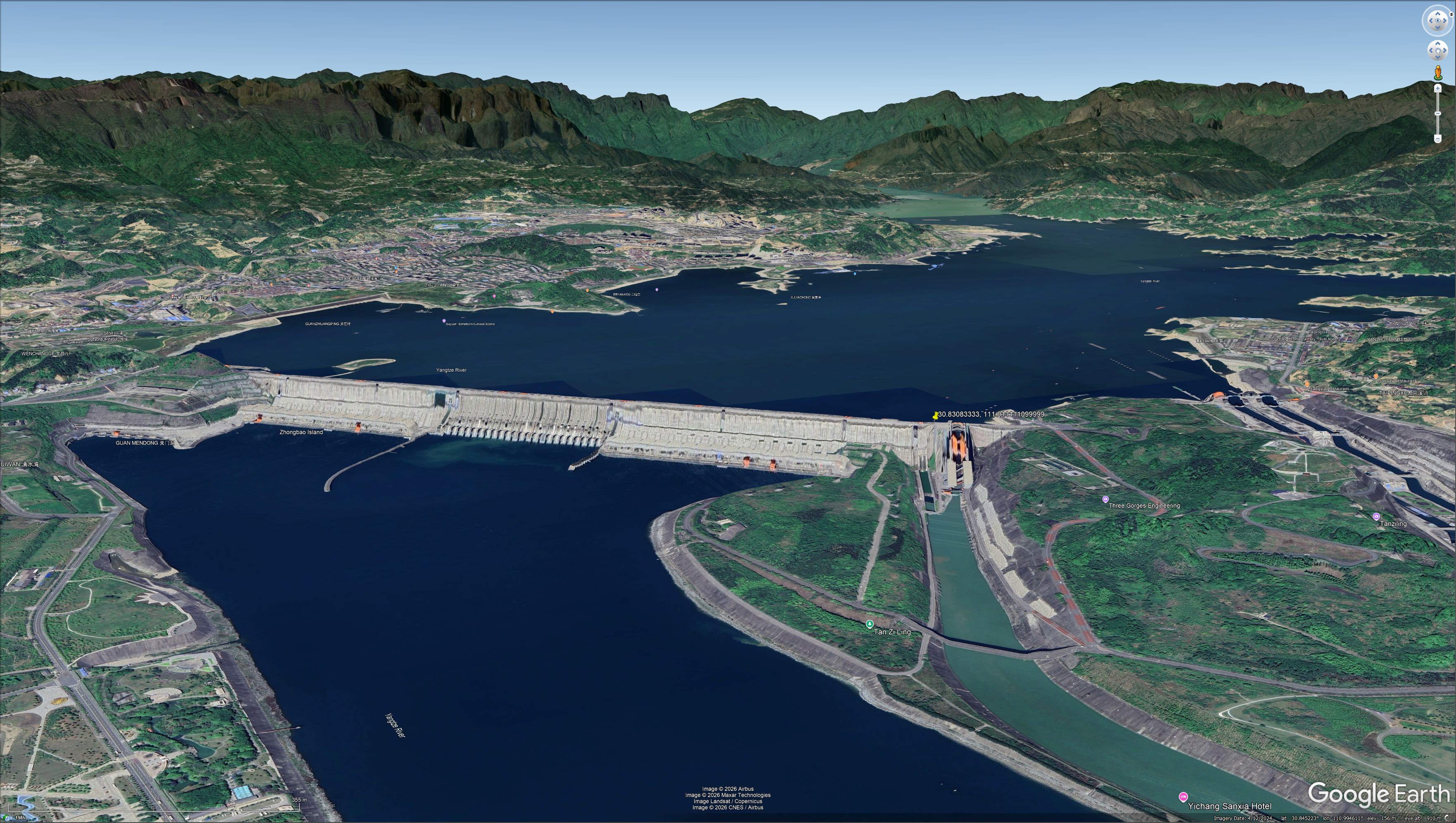
The following is a screenshot, taken from Google Earth, of the Three Gorges Dam, where the above station is located.
Below is a breakdown of unique values and NULL coverage across each column.
$ ~/duckdb
SELECT   column_name,
         column_type,
         null_percentage,
         approx_unique,
         min[:20],
         max[:20]
FROM     (SUMMARIZE
          SELECT * EXCLUDE(geometry)
          FROM   'hydro.parquet')
ORDER BY column_type,
         LOWER(column_name);
┌─────────────────────────────┬─────────────┬─────────────────┬───────────────┬──────────────────────┬──────────────────────┐
│         column_name         │ column_type │ null_percentage │ approx_unique │       min[:20]       │       max[:20]       │
│           varchar           │   varchar   │  decimal(9,2)   │     int64     │       varchar        │       varchar        │
├─────────────────────────────┼─────────────┼─────────────────┼───────────────┼──────────────────────┼──────────────────────┤
│ OGC_FID                     │ BIGINT      │            0.00 │          2943 │ 2                    │ 2919                 │
│ Annual_Power_Generation_MWh │ FLOAT       │           71.21 │           509 │ 0.00105              │ 882.0                │
│ Capacity_mw                 │ FLOAT       │           19.88 │           406 │ 0.0086               │ 60000.0              │
│ Dam_height_m                │ FLOAT       │           47.26 │           347 │ 2.05                 │ 325.0                │
│ Head_m                      │ FLOAT       │           56.13 │           546 │ 3.0                  │ 1184.0               │
│ Res_area_km2                │ FLOAT       │           48.46 │           805 │ 7.5e-05              │ 18800.0              │
│ Res_vol_Mm3                 │ FLOAT       │           61.38 │           661 │ 2.1e-06              │ 100000.0             │
│ Start_year                  │ INTEGER     │            8.84 │            95 │ 1909                 │ 2045                 │
│ Admin 1 (State/Province)    │ VARCHAR     │            0.00 │            32 │ Anhui                │ chekiang             │
│ Admin 2 (City/Region)       │ VARCHAR     │            0.14 │          1506 │ Aba Tibetan and Qian │ Zuogong              │
│ Feature ID                  │ VARCHAR     │            0.00 │          3310 │ GHN01                │ GHN999               │
│ Final_comments              │ VARCHAR     │           95.20 │            45 │ Actual name is Guang │ Uses tailwater from  │
│ Main_basin                  │ VARCHAR     │           60.76 │            45 │ Brahmaputra          │ Zi Shui              │
│ Name                        │ VARCHAR     │            0.00 │          2839 │ A Da                 │ Zuojiang Dam         │
│ River                       │ VARCHAR     │           17.44 │          1046 │ A Mo Jiang           │ longjiang River      │
│ Status                      │ VARCHAR     │           46.06 │             6 │ announced            │ shelved              │
│ Type                        │ VARCHAR     │            0.27 │             4 │ Mixed                │ Storage              │
│ Type_source                 │ VARCHAR     │            0.00 │             5 │ GEM                  │ manual               │
└─────────────────────────────┴─────────────┴─────────────────┴───────────────┴──────────────────────┴──────────────────────┘
Capacity Hotspots
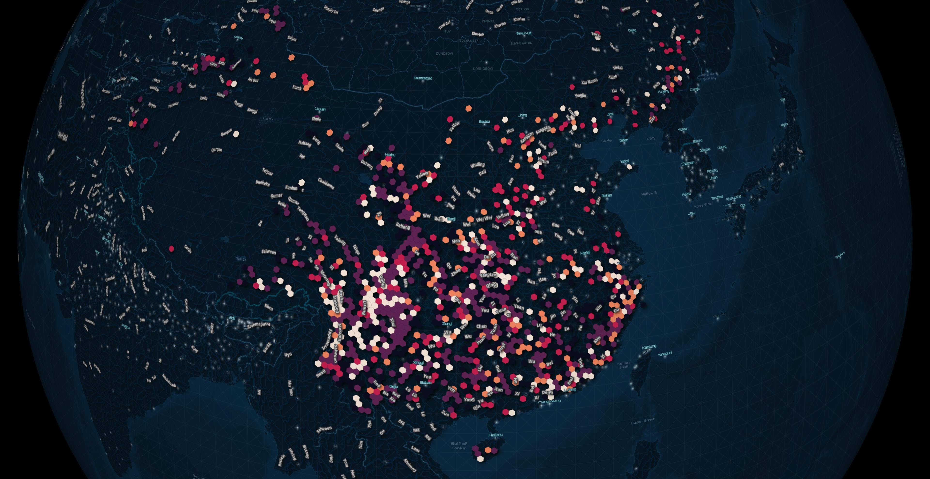
Below, I'll build a heatmap showing where station capacity, irrespective of status, is, was or will be at its greatest. The brighter the hexagon, the higher the capacity.
$ ~/duckdb
COPY (
    SELECT geometry: ST_ASWKB(H3_CELL_TO_BOUNDARY_WKT(hexagon)::geometry),
           Capacity_mw
    FROM   (

        SELECT   hexagon: H3_LATLNG_TO_CELL(
                            ST_Y(ST_GEOMFROMWKB(geometry)),
                            ST_X(ST_GEOMFROMWKB(geometry)),
                            4),
                 Capacity_mw: SUM(Capacity_mw)
        FROM     'hydro.parquet'
        GROUP BY 1)
) TO 'hydro_sum_capacity.h3_4s.parquet' (
        FORMAT 'PARQUET',
        CODEC  'ZSTD',
        COMPRESSION_LEVEL 22,
        ROW_GROUP_SIZE 15000);
This is a breakdown by decade of how much capacity each station is said to have had, rounded up to the nearest 4 GW.
Note: there are stations in this dataset that aren't expected to be built and operational until the middle of this century.
$ ~/duckdb -nullvalue ' '
PIVOT    (
    SELECT   decade:      ROUND(Start_year / 10)::INT * 10,
             Capacity_gw: CEIL(Capacity_mw / 4000)::INT * 4,
             cnt:         COUNT(*)
    FROM     'hydro.parquet'
    WHERE    decade BETWEEN 1940 AND 2050
    GROUP BY 1, 2
)
ON       Capacity_gw  IN (
            SELECT   DISTINCT CEIL(Capacity_mw / 4000)::INT * 4
            FROM     'hydro.parquet'
            ORDER BY 1)
USING    SUM(cnt)
GROUP BY decade
ORDER BY decade;
┌────────┬────────┬────────┬────────┬────────┬────────┬────────┬────────┐
│ decade │   4    │   8    │   12   │   16   │   24   │   44   │   60   │
│ int32  │ int128 │ int128 │ int128 │ int128 │ int128 │ int128 │ int128 │
├────────┼────────┼────────┼────────┼────────┼────────┼────────┼────────┤
│   1940 │      4 │        │        │        │        │        │        │
│   1950 │      2 │        │        │        │        │        │        │
│   1960 │     32 │        │        │        │        │        │        │
│   1970 │     41 │        │        │        │        │        │        │
│   1980 │     58 │        │        │        │        │        │        │
│   1990 │    122 │        │        │        │        │        │        │
│   2000 │    268 │        │        │        │        │        │        │
│   2010 │   1184 │      9 │        │        │      1 │        │        │
│   2020 │    229 │      2 │      2 │      4 │        │        │        │
│   2030 │    119 │        │        │        │        │        │        │
│   2040 │      6 │        │        │        │        │        │        │
│   2050 │        │        │        │        │        │        │      1 │
└────────┴────────┴────────┴────────┴────────┴────────┴────────┴────────┘
Of those stations under 4 GW of capacity, these are the station counts rounded to the nearest 400 MW.
PIVOT    (
    SELECT   decade:      ROUND(Start_year / 10)::INT * 10,
             Capacity_mw: CEIL(Capacity_mw / 400)::INT * 400,
             cnt:         COUNT(*)
    FROM     'hydro.parquet'
    WHERE    Capacity_mw < 4_000
    AND      decade IS NOT NULL
    GROUP BY 1, 2
)
ON       Capacity_mw  IN (
            SELECT   DISTINCT CEIL(Capacity_mw / 400)::INT * 400
            FROM     'hydro.parquet'
            WHERE    Capacity_mw < 4_000
            ORDER BY 1)
USING    SUM(cnt)
GROUP BY decade
ORDER BY decade;
┌────────┬────────┬────────┬────────┬────────┬────────┬────────┬────────┬────────┬────────┬────────┐
│ decade │  400   │  800   │  1200  │  1600  │  2000  │  2400  │  2800  │  3200  │  3600  │  4000  │
│ int32  │ int128 │ int128 │ int128 │ int128 │ int128 │ int128 │ int128 │ int128 │ int128 │ int128 │
├────────┼────────┼────────┼────────┼────────┼────────┼────────┼────────┼────────┼────────┼────────┤
│   1940 │      2 │      1 │        │      1 │        │        │        │        │        │        │
│   1950 │      1 │        │        │      1 │        │        │        │        │        │        │
│   1960 │     27 │        │      4 │        │      1 │        │        │        │        │        │
│   1970 │     31 │      2 │      6 │      1 │        │      1 │        │        │        │        │
│   1980 │     50 │      2 │      4 │      1 │      1 │        │        │        │        │        │
│   1990 │    106 │      8 │      3 │      1 │      1 │      2 │        │      1 │        │        │
│   2000 │    236 │     15 │      7 │      7 │      2 │        │        │        │      1 │        │
│   2010 │   1050 │     54 │     46 │      6 │     10 │     11 │      1 │      3 │      3 │        │
│   2020 │    124 │     31 │     33 │     18 │      7 │      5 │      4 │      5 │      1 │        │
│   2030 │     12 │      3 │     64 │     19 │      7 │     10 │      3 │        │        │        │
│   2040 │      4 │        │      1 │        │        │      1 │        │        │        │        │
└────────┴────────┴────────┴────────┴────────┴────────┴────────┴────────┴────────┴────────┴────────┘
This is the capacity ranking by river for stations that are currently operational.
SELECT   Capacity_GW: ROUND(SUM(Capacity_mw) / 1000)::INT,
         River
FROM     'hydro.parquet'
WHERE    River IS NOT NULL
AND      Status = 'operating'
GROUP BY 2
ORDER BY 1 DESC
LIMIT    25;
┌─────────────┬───────────────────────────────────────┐
│ Capacity_GW │                 River                 │
│    int32    │                varchar                │
├─────────────┼───────────────────────────────────────┤
│          33 │ Jinshajiang River                     │
│          25 │ Dadu River                            │
│          24 │ Yangtze                               │
│          24 │ Jinsha                                │
│          20 │ Mekong (Lancang)                      │
│          19 │ Yalong River                          │
│           8 │ Yellow River                          │
│           8 │ Salween (Nu)                          │
│           6 │ Lancang                               │
│           6 │ Wujiang River                         │
│           5 │ Huang He                              │
│           5 │ Chenledong                            │
│           5 │ Lancangjiang (Mekong) River           │
│           5 │ Yalongjiang River                     │
│           5 │ Yangtze (Jinsha)                      │
│           4 │ Luanhe River                          │
│           4 │ Dadu                                  │
│           4 │ Daxi Creek Branch of the Xitiao River │
│           3 │ Dadu He                               │
│           3 │ Lacang                                │
│           3 │ Min River                             │
│           3 │ Chang Jiang                           │
│           3 │ Yangtze (Tongtian)                    │
│           3 │ Dong River                            │
│           3 │ Mengjiang River                       │
└─────────────┴───────────────────────────────────────┘
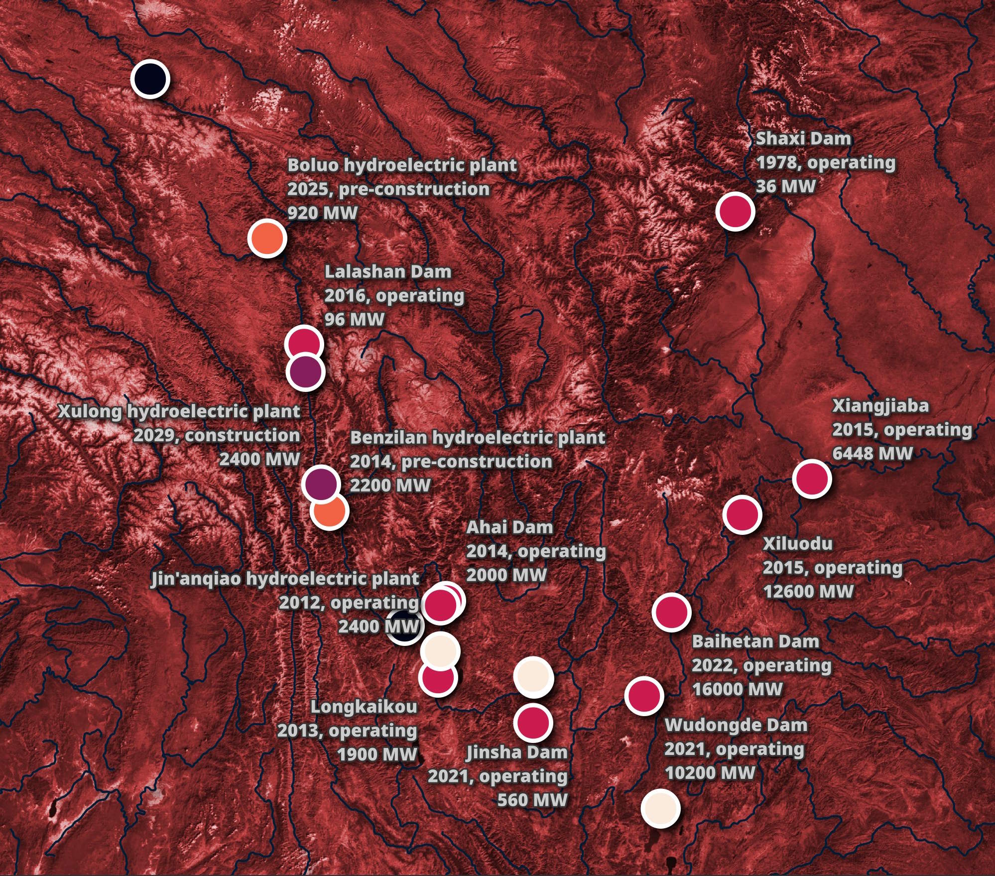
These are the locations of the Power Stations marked as being along either the Jinsha or Jinshajiang River.
Station Status
This is a breakdown of station status by decade.
$ ~/duckdb -nullvalue ' '
PIVOT (
    SELECT   decade: ROUND(Start_year / 10)::INT * 10,
             Status,
             cnt: COUNT(*)
    FROM     'hydro.parquet'
    WHERE    decade IS NOT NULL
    GROUP BY 1, 2
)
ON       Status
USING    SUM(cnt)
GROUP BY decade
ORDER BY decade;
┌────────┬───────────┬───────────┬──────────────┬───────────┬──────────────────┬─────────┐
│ decade │ announced │ cancelled │ construction │ operating │ pre-construction │ shelved │
│ int32  │  int128   │  int128   │    int128    │  int128   │      int128      │ int128  │
├────────┼───────────┼───────────┼──────────────┼───────────┼──────────────────┼─────────┤
│   1910 │           │           │              │         1 │                  │         │
│   1930 │           │           │              │           │                  │         │
│   1940 │           │           │              │         2 │                  │       1 │
│   1950 │           │           │              │         1 │                2 │       1 │
│   1960 │         2 │           │            5 │        24 │                6 │       1 │
│   1970 │         4 │           │            4 │        29 │                9 │         │
│   1980 │         2 │           │            3 │        45 │                3 │       1 │
│   1990 │         4 │           │            1 │       110 │                1 │       1 │
│   2000 │         3 │           │            1 │       207 │                4 │       2 │
│   2010 │         4 │           │           10 │       504 │               17 │       3 │
│   2020 │           │         1 │            5 │       156 │                5 │       2 │
│   2030 │         5 │         1 │           94 │         1 │               21 │         │
│   2040 │         2 │           │            1 │           │                3 │         │
│   2050 │           │           │              │           │                1 │         │
└────────┴───────────┴───────────┴──────────────┴───────────┴──────────────────┴─────────┘
Station Types
These are the station types broken down by the decade they were or are expected to be operational.
$ ~/duckdb -nullvalue ' '
PIVOT (
    SELECT   decade: ROUND(Start_year / 10)::INT * 10,
             Type,
             cnt: COUNT(*)
    FROM     'hydro.parquet'
    WHERE    decade IS NOT NULL
    GROUP BY 1, 2
)
ON       Type
USING    SUM(cnt)
GROUP BY decade
ORDER BY decade;
┌────────┬────────┬────────────────┬──────────────┬─────────┐
│ decade │ Mixed  │ Pumped Storage │ Run-of-River │ Storage │
│ int32  │ int128 │     int128     │    int128    │ int128  │
├────────┼────────┼────────────────┼──────────────┼─────────┤
│   1910 │        │                │            1 │         │
│   1930 │      1 │                │              │         │
│   1940 │      2 │                │            2 │       4 │
│   1950 │      2 │              3 │            2 │       1 │
│   1960 │    126 │             19 │           86 │      24 │
│   1970 │     84 │             17 │           60 │      31 │
│   1980 │     68 │              8 │           52 │      34 │
│   1990 │     43 │              9 │           49 │      51 │
│   2000 │     46 │             21 │           99 │     132 │
│   2010 │     56 │             52 │          699 │     399 │
│   2020 │      7 │             38 │           54 │     141 │
│   2030 │      2 │            101 │            2 │      17 │
│   2040 │      3 │                │            1 │       2 │
│   2050 │      1 │                │              │         │
└────────┴────────┴────────────────┴──────────────┴─────────┘
Dam Heights
These are the Dam heights, rounded up to the nearest 100 meters, broken down by the decade that they were or are expected to be operational. There is a trend towards taller heights in recent decades.
$ ~/duckdb -nullvalue ' '
PIVOT (
    SELECT   decade:       ROUND(Start_year / 10)::INT * 10,
             Dam_height_m: CEIL(Dam_height_m / 100)::INT * 100,
             cnt:          COUNT(*)
    FROM     'hydro.parquet'
    WHERE    decade IS NOT NULL
    GROUP BY 1, 2
)
ON       Dam_height_m
USING    SUM(cnt)
GROUP BY decade
ORDER BY decade;
┌────────┬────────┬────────┬────────┬────────┐
│ decade │  100   │  200   │  300   │  400   │
│ int32  │ int128 │ int128 │ int128 │ int128 │
├────────┼────────┼────────┼────────┼────────┤
│   1910 │      1 │        │        │        │
│   1930 │      1 │        │        │        │
│   1940 │      1 │      3 │        │        │
│   1950 │      6 │        │        │        │
│   1960 │    222 │      6 │        │        │
│   1970 │    168 │      5 │        │        │
│   1980 │    137 │      4 │        │        │
│   1990 │    105 │     10 │        │        │
│   2000 │    161 │     32 │      1 │        │
│   2010 │    391 │    115 │     19 │      4 │
│   2020 │     38 │     32 │     13 │      1 │
│   2030 │     15 │      5 │      3 │        │
│   2040 │      2 │        │        │      1 │
│   2050 │        │        │        │        │
└────────┴────────┴────────┴────────┴────────┘
Dam Head Heights
The Dam head height is the vertical distance between the water surface level at the intake and the water level at the point of discharge.
These are the station counts by head height, rounded to the nearest 200 meters, broken down by decade.
$ ~/duckdb -nullvalue ' '
PIVOT (
    SELECT   decade: ROUND(Start_year / 10)::INT * 10,
             Head_m: CEIL(Head_m / 200)::INT * 200,
             cnt:    COUNT(*)
    FROM     'hydro.parquet'
    WHERE    decade BETWEEN 1940 AND 2030
    GROUP BY 1, 2
)
ON       Head_m  IN (
            SELECT   DISTINCT CEIL(Head_m / 200)::INT * 200
            FROM     'hydro.parquet'
            ORDER BY 1)
USING    SUM(cnt)
GROUP BY decade
ORDER BY decade;
┌────────┬────────┬────────┬────────┬────────┬────────┬────────┐
│ decade │  200   │  400   │  600   │  800   │  1000  │  1200  │
│ int32  │ int128 │ int128 │ int128 │ int128 │ int128 │ int128 │
├────────┼────────┼────────┼────────┼────────┼────────┼────────┤
│   1940 │      3 │        │        │        │        │        │
│   1950 │        │        │        │        │        │        │
│   1960 │     12 │        │        │        │        │        │
│   1970 │     15 │        │      2 │        │        │        │
│   1980 │     32 │        │        │        │        │        │
│   1990 │     86 │      2 │      3 │        │        │        │
│   2000 │    145 │     12 │      3 │      2 │      1 │        │
│   2010 │    664 │    119 │     68 │     19 │      1 │      1 │
│   2020 │     39 │     16 │      6 │      2 │        │        │
│   2030 │      2 │      3 │        │        │        │        │
└────────┴────────┴────────┴────────┴────────┴────────┴────────┘
Reservoirs
These are the reservoir areas, rounded up to the nearest 500 KM2, broken down by decade.
$ ~/duckdb -nullvalue ' '
PIVOT (
    SELECT   decade:       ROUND(Start_year / 10)::INT * 10,
             Res_area_km2: CEIL(Res_area_km2 / 500)::INT * 500,
             cnt:          COUNT(*)
    FROM     'hydro.parquet'
    WHERE    decade < 2040
    GROUP BY 1, 2
)
ON       Res_area_km2  IN (
            SELECT   DISTINCT CEIL(Res_area_km2 / 500)::INT * 500
            FROM     'hydro.parquet'
            ORDER BY 1)
USING    SUM(cnt)
GROUP BY decade
ORDER BY decade;
┌────────┬────────┬────────┬────────┬────────┐
│ decade │  500   │  1000  │  1500  │ 19000  │
│ int32  │ int128 │ int128 │ int128 │ int128 │
├────────┼────────┼────────┼────────┼────────┤
│   1910 │      1 │        │        │        │
│   1930 │        │        │        │        │
│   1940 │      6 │        │        │        │
│   1950 │      6 │        │      1 │        │
│   1960 │    236 │        │        │        │
│   1970 │    173 │        │        │        │
│   1980 │    139 │        │        │        │
│   1990 │    111 │        │        │        │
│   2000 │    148 │      1 │        │        │
│   2010 │    601 │      1 │        │        │
│   2020 │     44 │        │        │      1 │
│   2030 │     14 │        │        │        │
└────────┴────────┴────────┴────────┴────────┘
These are the reservoir volumes, rounded up to the nearest 5,000 Mm3, broken down by decade.
PIVOT (
    SELECT   decade:      ROUND(Start_year / 10)::INT * 10,
             Res_vol_Mm3: CEIL(Res_vol_Mm3 / 5000)::INT * 5000,
             cnt:         COUNT(*)
    FROM     'hydro.parquet'
    WHERE    decade IS NOT NULL
    AND      decade < 2040
    GROUP BY 1, 2
)
ON       Res_vol_Mm3  IN (
            SELECT   DISTINCT CEIL(Res_vol_Mm3 / 5000)::INT * 5000
            FROM     'hydro.parquet'
            ORDER BY 1)
USING    SUM(cnt)
GROUP BY decade
ORDER BY decade;
┌────────┬────────┬────────┬────────┬────────┬────────┬────────┬────────┬────────┐
│ decade │  5000  │ 10000  │ 15000  │ 20000  │ 25000  │ 30000  │ 40000  │ 100000 │
│ int32  │ int128 │ int128 │ int128 │ int128 │ int128 │ int128 │ int128 │ int128 │
├────────┼────────┼────────┼────────┼────────┼────────┼────────┼────────┼────────┤
│   1910 │      1 │        │        │        │        │        │        │        │
│   1930 │        │        │        │        │        │        │        │        │
│   1940 │      3 │      1 │      2 │        │        │        │        │        │
│   1950 │      6 │        │      1 │        │        │        │        │        │
│   1960 │    228 │      2 │      1 │        │      1 │        │        │        │
│   1970 │    165 │      1 │        │        │      2 │        │        │        │
│   1980 │    131 │        │        │        │        │        │        │        │
│   1990 │    105 │      1 │        │        │        │      1 │        │        │
│   2000 │    137 │      1 │      1 │        │        │        │        │        │
│   2010 │    258 │      2 │      1 │        │      1 │      1 │      1 │        │
│   2020 │     33 │      1 │      1 │        │      1 │        │        │        │
│   2030 │     15 │        │        │        │        │        │        │        │
└────────┴────────┴────────┴────────┴────────┴────────┴────────┴────────┴────────┘