In November, Natural Resources Canada refreshed their Canadian Wind Turbine Database. It documents the location 7,841 wind turbines, their capabilities and associated project data across Canada.
In this post, I'll walk through converting this dataset into Parquet and examining some of its features.
My Workstation
I'm using a 5.7 GHz AMD Ryzen 9 9950X CPU. It has 16 cores and 32 threads and 1.2 MB of L1, 16 MB of L2 and 64 MB of L3 cache. It has a liquid cooler attached and is housed in a spacious, full-sized Cooler Master HAF 700 computer case.
The system has 96 GB of DDR5 RAM clocked at 4,800 MT/s and a 5th-generation, Crucial T700 4 TB NVMe M.2 SSD which can read at speeds up to 12,400 MB/s. There is a heatsink on the SSD to help keep its temperature down. This is my system's C drive.
The system is powered by a 1,200-watt, fully modular Corsair Power Supply and is sat on an ASRock X870E Nova 90 Motherboard.
I'm running Ubuntu 24 LTS via Microsoft's Ubuntu for Windows on Windows 11 Pro. In case you're wondering why I don't run a Linux-based desktop as my primary work environment, I'm still using an Nvidia GTX 1080 GPU which has better driver support on Windows and ArcGIS Pro only supports Windows natively.
Installing Prerequisites
I'll use jq to help analyse the data in this post.
$ sudo apt update
$ sudo apt install \
    jq
I'll use DuckDB, along with its H3, JSON, Lindel, Parquet and Spatial extensions in this post.
$ cd ~
$ wget -c https://github.com/duckdb/duckdb/releases/download/v1.5.0/duckdb_cli-linux-amd64.zip
$ unzip -j duckdb_cli-linux-amd64.zip
$ chmod +x duckdb
$ ~/duckdb
INSTALL h3 FROM community;
INSTALL lindel FROM community;
INSTALL json;
INSTALL parquet;
INSTALL spatial;
I'll set up DuckDB to load every installed extension each time it launches.
$ vi ~/.duckdbrc
.timer on
.width 180
LOAD h3;
LOAD lindel;
LOAD json;
LOAD parquet;
LOAD spatial;
Most of the maps in this post were rendered with QGIS version 4.0.0. QGIS is a desktop application that runs on Windows, macOS and Linux. The application has grown in popularity in recent years and has ~15M application launches from users all around the world each month.
I used QGIS' HCMGIS plugin to add basemaps from Esri to this post.
Downloading the Dataset
I'll download the dataset and convert it into Parquet.
$ mkdir -p ~/canada_wind
$ cd ~/canada_wind

$ wget https://ftp.cartes.canada.ca/pub/nrcan_rncan/Wind-energy_Energie-eolienne/wind_turbines_database/wind_turbine_database_en.gdb.zip
$ unzip -j wind_turbine_database_en.gdb.zip
$ ~/duckdb
COPY (
    SELECT * EXCLUDE(SHAPE,
                     Longitude,
                     Latitude,
                     Turbine_Rated_Capacity_kW,
                     Total_Project_Capacity_MW,
                     Number_of_Turbines_in_Project,
                     Turbine_Number,
                     Rotor_Diameter_m,
                     Commissioning,
                     Hub_Height_m),
           commissioning:             SPLIT(Commissioning, '/')[1]::INT,
           Turbine_Rated_Capacity_kW: SPLIT(SPLIT(Turbine_Rated_Capacity_kW, '/')[1], '-')[1]::FLOAT,
           Hub_Height_m:              SPLIT(Hub_Height_m, '-')[1]::FLOAT,
           Number_of_Turbines_in_Project:
                                      Number_of_Turbines_in_Project::INT,
           Rotor_Diameter_m:          Rotor_Diameter_m::FLOAT,
           Total_Project_Capacity_MW: Total_Project_Capacity_MW::FLOAT,
           Turbine_Number:            Turbine_Number::INT,

           geometry:                  ST_POINT(Longitude,
                                               Latitude),
           bbox:                      {'xmin': ST_XMIN(ST_EXTENT(geometry)),
                                       'ymin': ST_YMIN(ST_EXTENT(geometry)),
                                       'xmax': ST_XMAX(ST_EXTENT(geometry)),
                                       'ymax': ST_YMAX(ST_EXTENT(geometry))}
    FROM     ST_READ('a00000009.gdbtable')
    ORDER BY HILBERT_ENCODE([ST_Y(ST_CENTROID(geometry)),
                             ST_X(ST_CENTROID(geometry))]::double[2])
) TO 'wind.parquet' (
        FORMAT 'PARQUET',
        CODEC  'ZSTD',
        COMPRESSION_LEVEL 22,
        ROW_GROUP_SIZE 15000);
The above produced a 316 KB Parquet file containing 7,841 rows.
Data Fluency
The following is an example record from this dataset.
$ echo "FROM 'wind.parquet'
        LIMIT 1" \
    | ~/duckdb -json \
    | jq -S .
[
  {
    "Hub_Height_m": 50.0,
    "Manufacturer": "Vestas",
    "Model": "V47-660",
    "Notes": "",
    "Number_of_Turbines_in_Project": 16,
    "Project_Name": "North Cape Wind Farm Phase",
    "Province_Territory": "Prince Edward Island",
    "Rotor_Diameter_m": 47.0,
    "Total_Project_Capacity_MW": 10.5600004196167,
    "Turbine_Identifier": "NCW7",
    "Turbine_Number": 7,
    "Turbine_Rated_Capacity_kW": 660.0,
    "bbox": {
      "xmax": -63.9950147,
      "xmin": -63.9950147,
      "ymax": 47.0485158,
      "ymin": 47.0485158
    },
    "commissioning": 2001,
    "geometry": "POINT (-63.9950147 47.0485158)"
  }
]
Below are the field names, data types, percentages of NULLs per column, number of unique values and minimum and maximum values for each column.
$ ~/duckdb
SELECT   column_name,
         column_type[:30],
         null_percentage,
         approx_unique,
         min[:30],
         max[:30]
FROM     (SUMMARIZE
          FROM 'wind.parquet')
ORDER BY LOWER(column_name);
┌───────────────────────────────┬────────────────────────────────┬─────────────────┬───────────────┬────────────────────────────────┬────────────────────────────────┐
│          column_name          │        column_type[:30]        │ null_percentage │ approx_unique │            min[:30]            │            max[:30]            │
│            varchar            │            varchar             │  decimal(9,2)   │     int64     │            varchar             │            varchar             │
├───────────────────────────────┼────────────────────────────────┼─────────────────┼───────────────┼────────────────────────────────┼────────────────────────────────┤
│ bbox                          │ STRUCT(xmin DOUBLE, ymin DOUBL │            0.00 │          8837 │ {'xmin': -138.841952, 'ymin':  │ {'xmin': -52.970072, 'ymin': 4 │
│ commissioning                 │ INTEGER                        │            0.00 │            30 │ 1993                           │ 2025                           │
│ geometry                      │ GEOMETRY('OGC:CRS84')          │            0.00 │          7466 │ POINT (-82.29153133 42.2526119 │ POINT (-107.177635 50.31832261 │
│ Hub_Height_m                  │ FLOAT                          │            0.00 │            62 │ 15.2                           │ 150.0                          │
│ Manufacturer                  │ VARCHAR                        │            0.00 │            35 │ Acciona Wind Power             │ Windmatic                      │
│ Model                         │ VARCHAR                        │            0.00 │           109 │ 25xc                           │ WM15S                          │
│ Notes                         │ VARCHAR                        │            0.00 │            79 │                                │ Vertical Axis Hybrid           │
│ Number_of_Turbines_in_Project │ INTEGER                        │            0.00 │            71 │ 1                              │ 175                            │
│ Project_Name                  │ VARCHAR                        │            0.00 │           294 │ Adelaide Wind Energy Centre    │ Zurich                         │
│ Province_Territory            │ VARCHAR                        │            0.00 │            12 │ Alberta                        │ Yukon                          │
│ Rotor_Diameter_m              │ FLOAT                          │            0.00 │            59 │ 1.93                           │ 170.0                          │
│ Total_Project_Capacity_MW     │ FLOAT                          │            0.00 │           195 │ 0.0                            │ 494.0                          │
│ Turbine_Identifier            │ VARCHAR                        │            0.00 │          8495 │ AAV1                           │ ZUR1                           │
│ Turbine_Number                │ INTEGER                        │            0.00 │           184 │ 1                              │ 175                            │
│ Turbine_Rated_Capacity_kW     │ FLOAT                          │            0.00 │            66 │ 0.0                            │ 6600.0                         │
└───────────────────────────────┴────────────────────────────────┴─────────────────┴───────────────┴────────────────────────────────┴────────────────────────────────┘
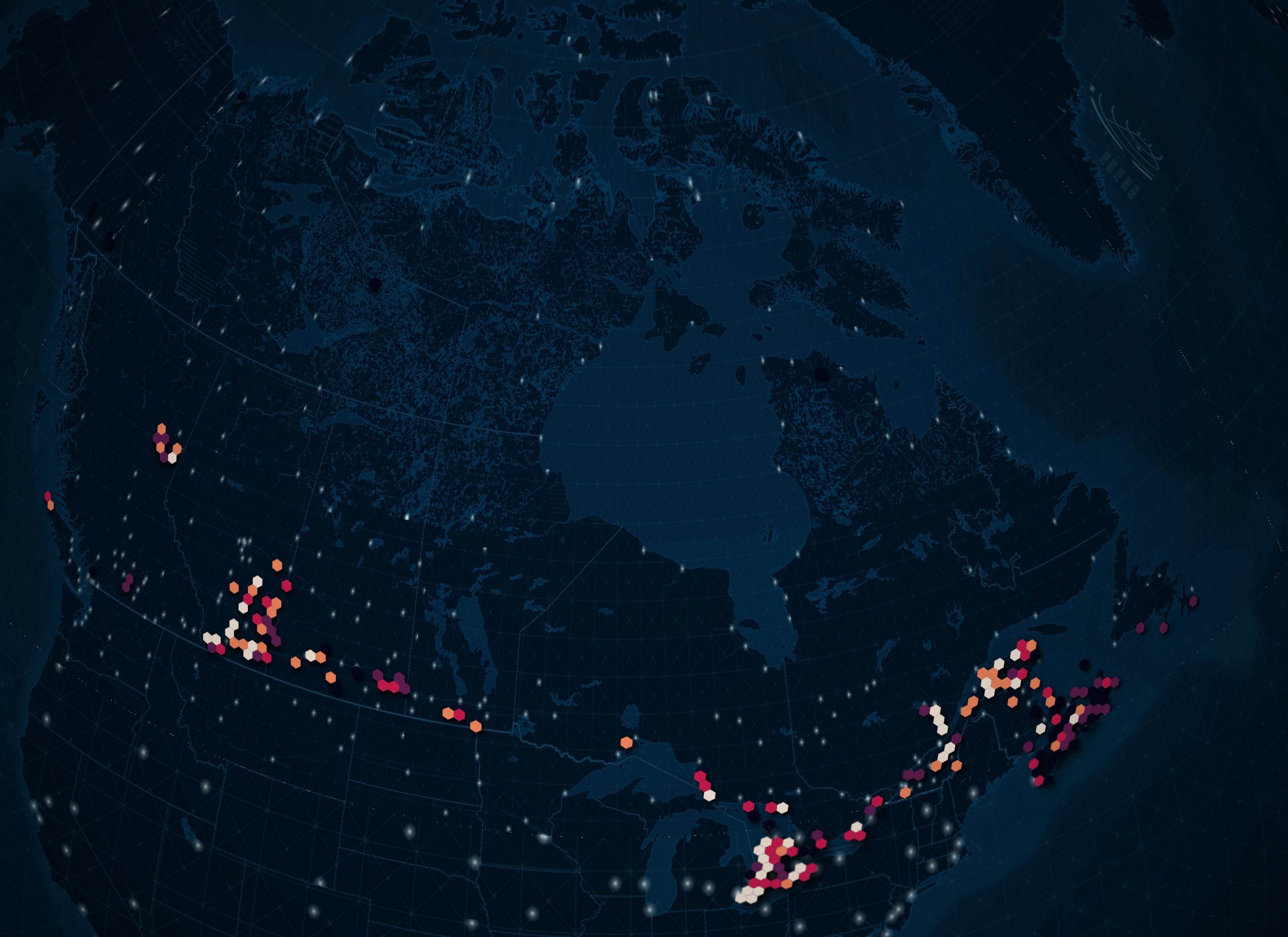
Turbines
Below I'll generate a heatmap of turbine installation locations.
$ ~/duckdb
CREATE OR REPLACE TABLE h3_4_stats AS
    SELECT   h3_4: H3_LATLNG_TO_CELL(
                        bbox.ymin,
                        bbox.xmin,
                        4),
             COUNT(*) num_turbines
    FROM     'wind.parquet'
    GROUP BY 1;

COPY (
    SELECT geometry: ST_ASWKB(H3_CELL_TO_BOUNDARY_WKT(h3_4)::geometry),
           num_turbines
    FROM   h3_4_stats
) TO 'turbines.h3_4.parquet' (
        FORMAT 'PARQUET',
        CODEC  'ZSTD',
        COMPRESSION_LEVEL 22,
        ROW_GROUP_SIZE 15000);
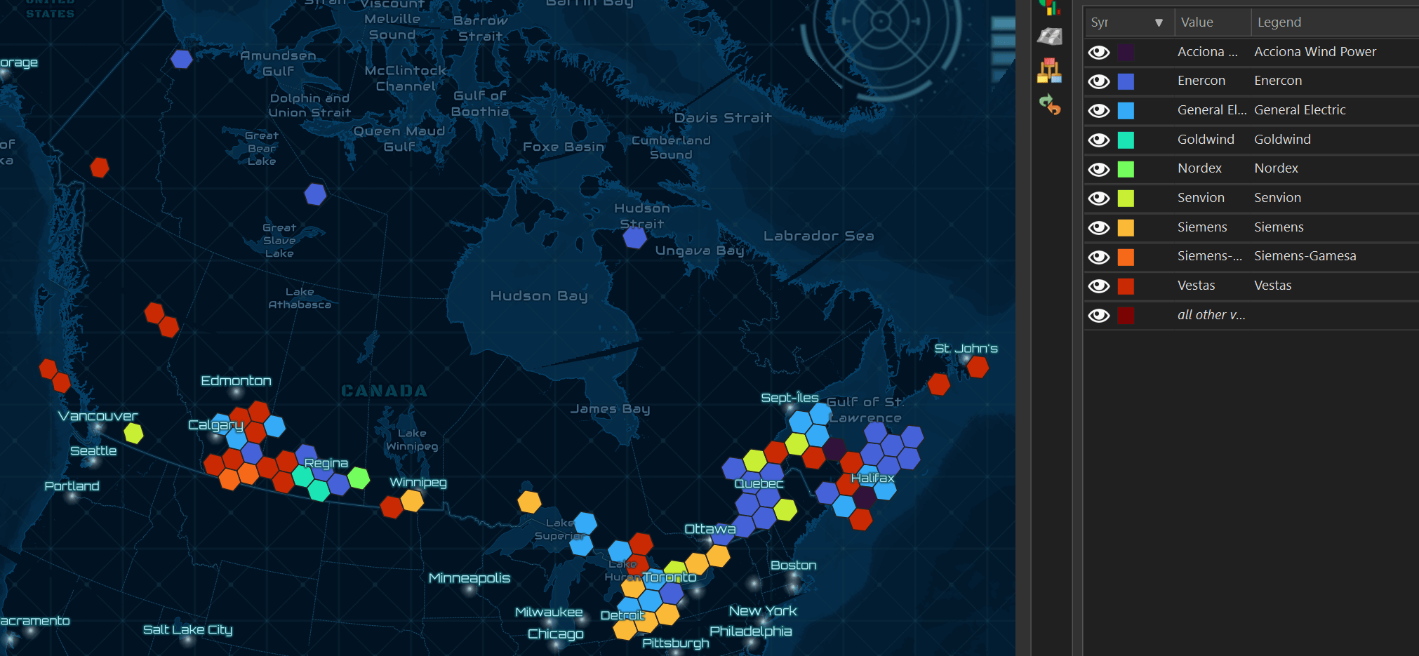
There are 34 unique manufactures listed in this dataset. These are the ones with the most and least number of turbines installed.
$ ~/duckdb
SELECT   num_turbines: COUNT(*),
         Manufacturer
FROM     'wind.parquet'
GROUP BY 2
ORDER BY 1 DESC;
┌──────────────┬──────────────────────────┐
│ num_turbines │       Manufacturer       │
│    int64     │         varchar          │
├──────────────┼──────────────────────────┤
│         2173 │ Vestas                   │
│         1726 │ General Electric         │
│         1247 │ Siemens                  │
│         1092 │ Enercon                  │
│          643 │ Senvion                  │
│          491 │ Siemens-Gamesa           │
│          132 │ NEG Micon                │
│          105 │ Nordex                   │
│           74 │ Acciona Wind Power       │
│           50 │ Goldwind                 │
│           16 │ Ghrepower                │
│           15 │ Suzlon                   │
│           12 │ Seaforth                 │
│            9 │ Vensys                   │
│            8 │ Gamesa                   │
│            7 │ Endurance Wind Power     │
│            6 │ Windmatic                │
│            5 │ DeWind                   │
│            5 │ EWT                      │
│            4 │ Samsung Renewable Energy │
│            3 │ Northwind                │
│            3 │ Turbowinds               │
│            2 │ Bonus                    │
│            2 │ America Wind Energy      │
│            2 │ Lagerwey                 │
│            1 │ Pfleiderer               │
│            1 │ Bergey                   │
│            1 │ Tacke                    │
│            1 │ Leitwind                 │
│            1 │ Enercon                  │
│            1 │ Neg Micon                │
│            1 │ Wind Energy Solutions    │
│            1 │ Southwest Windpower      │
│            1 │ Darrieus-Savonius        │
└──────────────┴──────────────────────────┘
Below are the number of turbines by manufacturer commissioned by decade.
WITH a AS (
    SELECT   num_turbines: COUNT(*),
             decade:       (Commissioning / 10)::INT * 10,
             manufacturer: Manufacturer
    FROM     'wind.parquet'
    GROUP BY 2, 3
    ORDER BY 1 DESC
)
PIVOT    a
ON       decade
USING    SUM(num_turbines)
GROUP BY manufacturer
ORDER BY manufacturer;
┌──────────────────────────┬────────┬────────┬────────┬────────┐
│       manufacturer       │  1990  │  2000  │  2010  │  2020  │
│         varchar          │ int128 │ int128 │ int128 │ int128 │
├──────────────────────────┼────────┼────────┼────────┼────────┤
│ Acciona Wind Power       │   NULL │   NULL │     40 │     34 │
│ America Wind Energy      │   NULL │   NULL │      2 │   NULL │
│ Bergey                   │   NULL │   NULL │      1 │   NULL │
│ Bonus                    │      2 │   NULL │   NULL │   NULL │
│ Darrieus-Savonius        │   NULL │   NULL │   NULL │      1 │
│ DeWind                   │   NULL │   NULL │      5 │   NULL │
│ EWT                      │   NULL │   NULL │   NULL │      5 │
│ Endurance Wind Power     │   NULL │   NULL │      3 │      4 │
│ Enercon                  │   NULL │      3 │    796 │    293 │
│ Enercon                  │   NULL │   NULL │   NULL │      1 │
│ Gamesa                   │   NULL │   NULL │      8 │   NULL │
│ General Electric         │   NULL │     20 │   1460 │    246 │
│ Ghrepower                │   NULL │   NULL │      2 │     14 │
│ Goldwind                 │   NULL │   NULL │   NULL │     50 │
│ Lagerwey                 │   NULL │      2 │   NULL │   NULL │
│ Leitwind                 │   NULL │   NULL │      1 │   NULL │
│ NEG Micon                │   NULL │    132 │   NULL │   NULL │
│ Neg Micon                │   NULL │      1 │   NULL │   NULL │
│ Nordex                   │   NULL │     20 │   NULL │     85 │
│ Northwind                │   NULL │   NULL │      3 │   NULL │
│ Pfleiderer               │   NULL │   NULL │      1 │   NULL │
│ Samsung Renewable Energy │   NULL │   NULL │      4 │   NULL │
│ Seaforth                 │   NULL │   NULL │     12 │   NULL │
│ Senvion                  │   NULL │   NULL │    488 │    155 │
│ Siemens                  │   NULL │   NULL │    710 │    537 │
│ Siemens-Gamesa           │   NULL │   NULL │   NULL │    491 │
│ Southwest Windpower      │   NULL │   NULL │      1 │   NULL │
│ Suzlon                   │   NULL │   NULL │     15 │   NULL │
│ Tacke                    │   NULL │      1 │   NULL │   NULL │
│ Turbowinds               │   NULL │      3 │   NULL │   NULL │
│ Vensys                   │   NULL │      1 │      8 │   NULL │
│ Vestas                   │   NULL │    421 │   1239 │    513 │
│ Wind Energy Solutions    │   NULL │   NULL │      1 │   NULL │
│ Windmatic                │   NULL │      6 │   NULL │   NULL │
└──────────────────────────┴────────┴────────┴────────┴────────┘
Below I'll plot out the top manufacturer per hexagon among the overall top ten.
CREATE OR REPLACE TABLE top_manufacturers AS
    SELECT   num_turbines: COUNT(*),
             manufacturer: Manufacturer
    FROM     'wind.parquet'
    GROUP BY 2
    ORDER BY 1 DESC
    LIMIT    10;

CREATE OR REPLACE TABLE h3_3s AS
    WITH b AS (
        WITH a AS (
            SELECT   h3_3: H3_LATLNG_TO_CELL(
                                bbox.ymin,
                                bbox.xmin,
                                3) ,
                     manufacturer: Manufacturer,
                     num_recs: COUNT(*)
            FROM     'wind.parquet'
            WHERE    Manufacturer IN (
                SELECT DISTINCT manufacturer
                FROM   top_manufacturers
            )
            GROUP BY 1, 2
        )
        SELECT *,
               ROW_NUMBER() OVER (PARTITION BY h3_3
                                  ORDER BY     num_recs DESC) AS rn
        FROM   a
    )
    FROM     b
    WHERE    rn = 1
    ORDER BY num_recs DESC;

COPY (
    SELECT geom: H3_CELL_TO_BOUNDARY_WKT(h3_3)::GEOMETRY,
           manufacturer
    FROM   h3_3s
) TO 'turbine.top_manufacturer.h3_3.parquet' (
    FORMAT 'PARQUET',
    CODEC  'ZSTD',
    COMPRESSION_LEVEL 22,
    ROW_GROUP_SIZE 15000);
Below are the provinces and territories ranked by their total GW of installed capacity along with the number of turbines and distinct manufacturers represented.
SELECT   Province_Territory,
         gw:                ROUND(SUM(Turbine_Rated_Capacity_kW / 1000 ** 2), 3),
         num_turbines:      COUNT(*),
         num_manufacturers: COUNT(DISTINCT Manufacturer)
FROM     'wind.parquet'
GROUP BY 1
ORDER BY 2 DESC
LIMIT    20;
┌───────────────────────────┬────────┬──────────────┬───────────────────┐
│    Province_Territory     │   gw   │ num_turbines │ num_manufacturers │
│          varchar          │ double │    int64     │       int64       │
├───────────────────────────┼────────┼──────────────┼───────────────────┤
│ Alberta                   │   5.77 │         1778 │                10 │
│ Ontario                   │   5.55 │         2712 │                14 │
│ Quebec                    │  3.933 │         2005 │                 6 │
│ Saskatchewan              │  0.821 │          277 │                 6 │
│ British Columbia          │  0.747 │          300 │                 5 │
│ Nova Scotia               │  0.622 │          347 │                11 │
│ New Brunswick             │  0.422 │          146 │                 4 │
│ Manitoba                  │  0.258 │          133 │                 2 │
│ Prince Edward Island      │  0.201 │          104 │                 3 │
│ Newfoundland and Labrador │  0.055 │           27 │                 3 │
│ Northwest Territories     │  0.013 │            5 │                 1 │
│ Yukon                     │  0.005 │            7 │                 3 │
└───────────────────────────┴────────┴──────────────┴───────────────────┘
Below shows the ever-increasing capacity of turbines in MW over the decades.
WITH a AS (
    SELECT   decade:       (commissioning / 10)::INT * 10,
             mw:           CEIL(Turbine_Rated_Capacity_kW / 1000),
             num_turbines: COUNT(*)
    FROM     'wind.parquet'
    GROUP BY 1, 2
)
PIVOT    a
ON       decade
USING    SUM(num_turbines)
GROUP BY mw
ORDER BY mw;
┌───────┬────────┬────────┬────────┬────────┐
│  mw   │  1990  │  2000  │  2010  │  2020  │
│ float │ int128 │ int128 │ int128 │ int128 │
├───────┼────────┼────────┼────────┼────────┤
│   0.0 │      1 │     24 │      3 │   NULL │
│   1.0 │      1 │    358 │     37 │     26 │
│   2.0 │   NULL │    226 │   3160 │    469 │
│   3.0 │   NULL │      2 │   1600 │    500 │
│   4.0 │   NULL │   NULL │   NULL │    569 │
│   5.0 │   NULL │   NULL │   NULL │    529 │
│   6.0 │   NULL │   NULL │   NULL │    269 │
│   7.0 │   NULL │   NULL │   NULL │     67 │
└───────┴────────┴────────┴────────┴────────┘
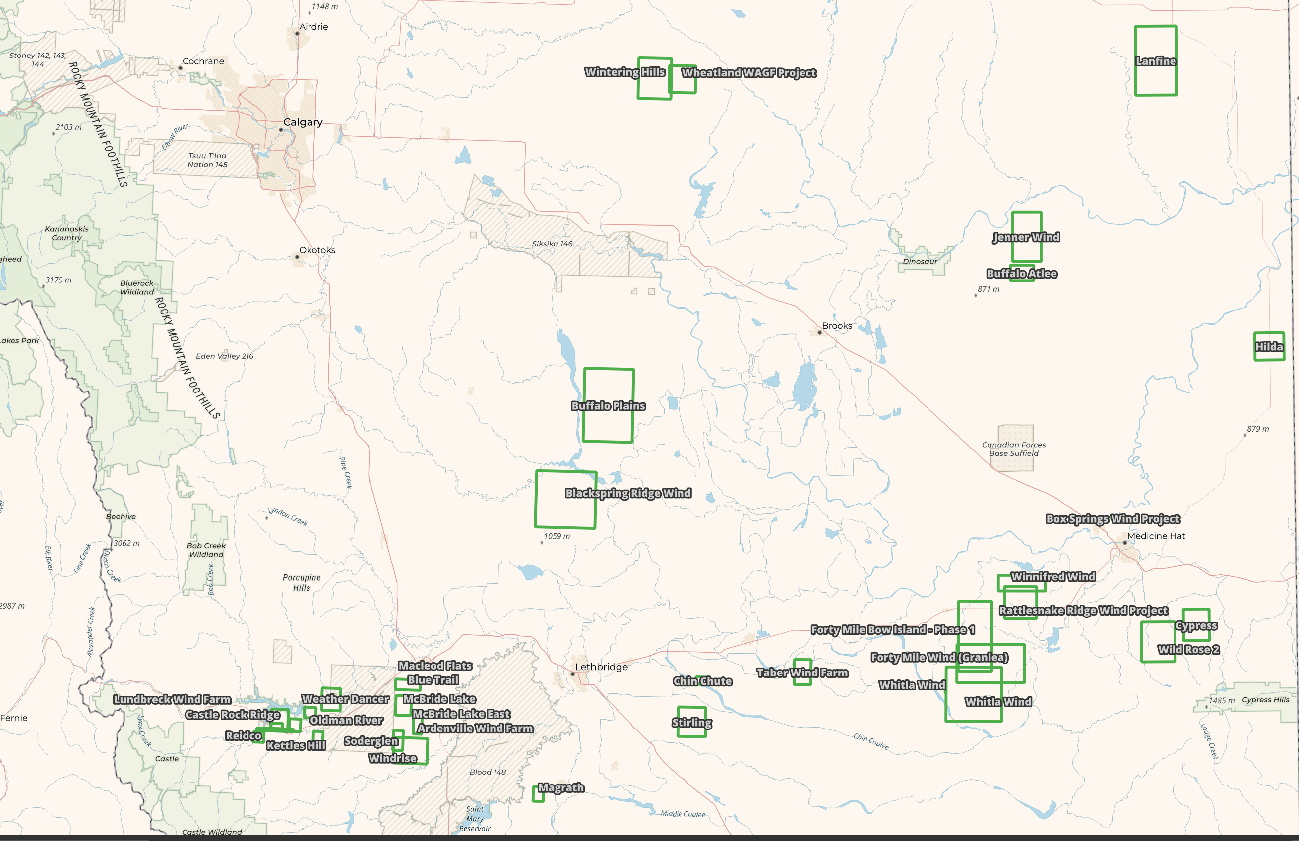
Project Footprints
Each turbine record contains a project name. Below I'll generate the footprints for each project.
I'll group the projects by hexagon and name to generate their geographical footprints. This helps avoid country-wide overlaps that would result from grouping by name alone.
$ ~/duckdb
COPY (
    SELECT   h3_3: H3_LATLNG_TO_CELL(bbox.ymin,
                                     bbox.xmin,
                                     2),
             project_name: Project_Name,
             geometry: {
                'min_x': MIN(ST_X(geometry)),
                'min_y': MIN(ST_Y(geometry)),
                'max_x': MAX(ST_X(geometry)),
                'max_y': MAX(ST_Y(geometry))}::BOX_2D::GEOMETRY
    FROM     READ_PARQUET('wind.parquet')
    GROUP BY 1, 2
) TO 'projects.parquet' (
        FORMAT 'PARQUET',
        CODEC  'ZSTD',
        COMPRESSION_LEVEL 22,
        ROW_GROUP_SIZE 15000);
A total of 327 distinct projects were returned. Below are a few of these projects in southern Alberta.