Canada has been running a satellite programme called RADARSAT since the 1990s. The first constellation was launched in 1995, the second in 2007 and the third (RCM) in 2019.
The three satellites in the RCM constellation capture Synthetic Aperture Radar (SAR) imagery as well as AIS tracking data from ships. SAR allows for imagery to be taken day or night and can see through clouds and through some types of camouflage. It can also be used to classify the materials it captures. I'm not sure if RCM supports this, but commercial SAR operators can also capture video, not just still imagery.
The constellation is primarily used for maritime surveillance, disaster management, climate research as well as oil exploration. They can capture imagery from 95% of the Earth's surface on any given day.
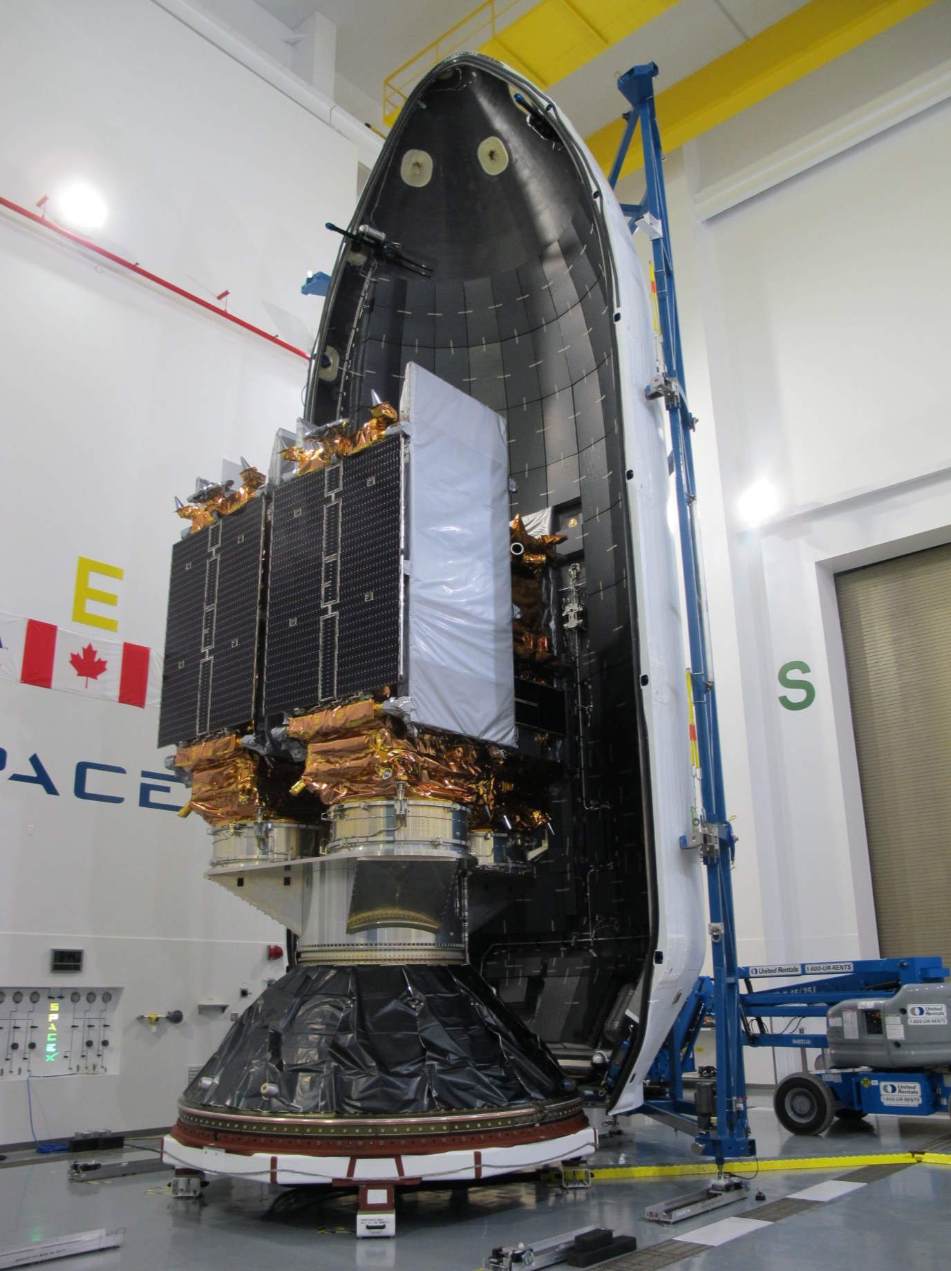
This image shows the satellites getting ready for launch in June, 2019.
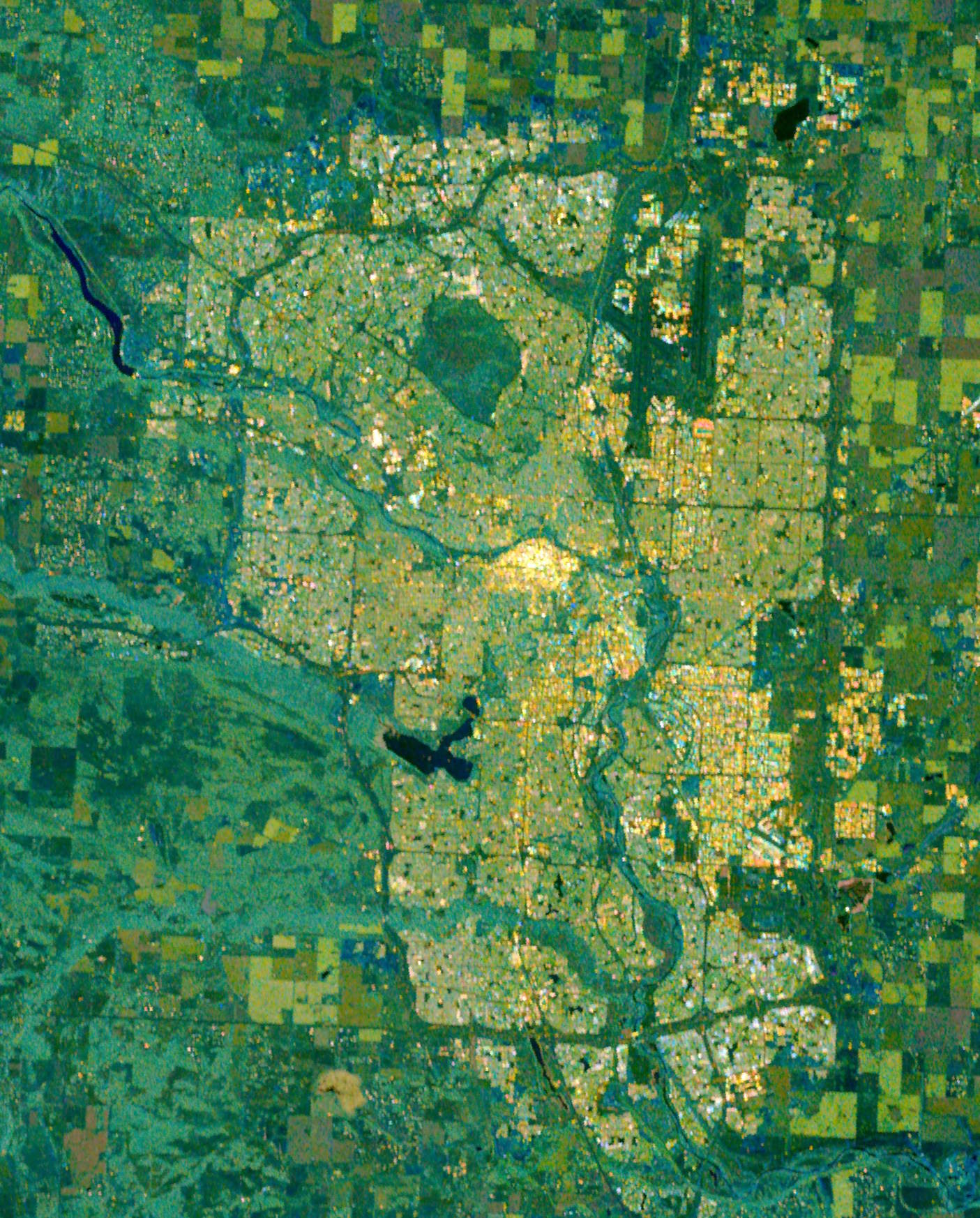
Below is a screenshot of a 96 GB, Cloud-Optimised GeoTIFF mosaic of RCM's imagery of Canada.

Below, I've zoomed in on Calgary.
These are the latest constellation details from GCAT.
$ ~/duckdb
SELECT   Name,
         JCAT,
         Manufacturer,
         Owner,
         LDate,
         Launch_Tag,
         Bus,
         Shape,
         DryMass,
         Length,
         Diameter,
         Span,
         TotMass,
         OpOrbit,
         Apogee,
         Inc,
         Perigee,
         Status
FROM     'gcat/satcat.parquet'
WHERE    NAME ILIKE 'RCM%'
ORDER BY Launch_Tag,
         Name;
┌─────────┬─────────┬──────────────┬─────────┬─────────────┬────────────┬─────────┬──────────────┬─────────┬────────┬──────────┬───────┬─────────┬─────────┬────────┬───────┬─────────┬──────────┐
│  Name   │  JCAT   │ Manufacturer │  Owner  │    LDate    │ Launch_Tag │   Bus   │    Shape     │ DryMass │ Length │ Diameter │ Span  │ TotMass │ OpOrbit │ Apogee │  Inc  │ Perigee │  Status  │
│ varchar │ varchar │   varchar    │ varchar │   varchar   │  varchar   │ varchar │   varchar    │ varchar │ float  │  float   │ float │  float  │ varchar │ int32  │ float │ varchar │ varchar  │
├─────────┼─────────┼──────────────┼─────────┼─────────────┼────────────┼─────────┼──────────────┼─────────┼────────┼──────────┼───────┼─────────┼─────────┼────────┼───────┼─────────┼──────────┤
│ RCM 1   │ S44322  │ BALM/MAXAR   │ CSA     │ 2019 Jun 12 │ 2019-033   │ MAC-200 │ Box+2 panels │ 1400    │    5.0 │      1.4 │   7.0 │  1450.0 │ LLEO/S  │    604 │ 97.77 │ 584     │ In orbit │
│ RCM 2   │ S44323  │ BALM/MAXAR   │ CSA     │ 2019 Jun 12 │ 2019-033   │ MAC-200 │ Box+2 panels │ 1400    │    5.0 │      1.4 │   7.0 │  1450.0 │ LLEO/S  │    603 │ 97.77 │ 584     │ In orbit │
│ RCM 3   │ S44324  │ BALM/MAXAR   │ CSA     │ 2019 Jun 12 │ 2019-033   │ MAC-200 │ Box+2 panels │ 1400    │    5.0 │      1.4 │   7.0 │  1450.0 │ LLEO/S  │    603 │ 97.77 │ 584     │ In orbit │
└─────────┴─────────┴──────────────┴─────────┴─────────────┴────────────┴─────────┴──────────────┴─────────┴────────┴──────────┴───────┴─────────┴─────────┴────────┴───────┴─────────┴──────────┘
Natural Resources Canada publishes its RCM imagery capture plans every two weeks. Over the summer, I've been archiving these.
In this post, I'll clean up and analyse the SAR footprints and associated metadata documented in their plans.
I'd like to give a special thanks to Max Lenormand for helping me put this post together. Max previously worked for ICEYE, a commercial SAR satellite manufacturer and constellation operator, based in Finland. Two years ago, Max published a well-received introduction to SAR video on YouTube.
My Workstation
I'm using a 5.7 GHz AMD Ryzen 9 9950X CPU. It has 16 cores and 32 threads and 1.2 MB of L1, 16 MB of L2 and 64 MB of L3 cache. It has a liquid cooler attached and is housed in a spacious, full-sized Cooler Master HAF 700 computer case.
The system has 96 GB of DDR5 RAM clocked at 4,800 MT/s and a 5th-generation, Crucial T700 4 TB NVMe M.2 SSD which can read at speeds up to 12,400 MB/s. There is a heatsink on the SSD to help keep its temperature down. This is my system's C drive.
The system is powered by a 1,200-watt, fully modular Corsair Power Supply and is sat on an ASRock X870E Nova 90 Motherboard.
I'm running Ubuntu 24 LTS via Microsoft's Ubuntu for Windows on Windows 11 Pro. In case you're wondering why I don't run a Linux-based desktop as my primary work environment, I'm still using an Nvidia GTX 1080 GPU which has better driver support on Windows and ArcGIS Pro only supports Windows natively.
Installing Prerequisites
I'll use jq to help format some data in this post.
$ sudo apt update
$ sudo apt install \
    jq
I'll be using JSON Convert (jc) to convert the output of various CLI tools into JSON.
$ wget https://github.com/kellyjonbrazil/jc/releases/download/v1.25.2/jc_1.25.2-1_amd64.deb
$ sudo dpkg -i jc_1.25.2-1_amd64.deb
I'll use DuckDB, along with its H3, JSON, Lindel, Parquet and Spatial extensions in this post.
$ cd ~
$ wget -c https://github.com/duckdb/duckdb/releases/download/v1.5.4/duckdb_cli-linux-amd64.zip
$ unzip -j duckdb_cli-linux-amd64.zip
$ chmod +x duckdb
$ ~/duckdb
INSTALL h3 FROM community;
INSTALL lindel FROM community;
INSTALL json;
INSTALL parquet;
INSTALL spatial;
I'll set up DuckDB to load every installed extension each time it launches.
$ vi ~/.duckdbrc
.timer on
.width 180
LOAD h3;
LOAD lindel;
LOAD json;
LOAD parquet;
LOAD spatial;
The maps in this post were rendered with QGIS version 4.2.1. QGIS is a desktop application that runs on Windows, macOS and Linux. The application has grown in popularity in recent years and has ~22M application launches from users all around the world each month.
The boundaries and place names were sourced from Natural Earth. The Arctic Sea Routes were sourced from the National Geospatial-Intelligence Agency. Maritime Boundaries were sourced from Marine Regions. I used QGIS' HCMGIS plugin to add satellite imagery basemaps from Bing and Esri to this post.
Analysis-Ready Data
The mission plan URLs and filenames aren't versioned. When a new plan is published, the previous plan is no longer publicly available.
I'm running a weekly cron job that fetches the last modified time of the ZIP file. That timestamp forms part of the filename where I store it locally. If the filename exists and has already been fully downloaded, wget will report that there isn't anything more to download. But if the filename doesn't exist locally, it will download the ZIP file.
The following is the BASH script my cron job would call.
URL=https://ftp.maps.canada.ca/pub/csa_asc/Space-technology_Technologie-spatiale/radarsat_constellation_mission_plan/radarsat_constellation_mission_planned.shp.zip

TIMESTAMP=`curl -sI "$URL" | jc --kv | jq -r '."Last-Modified"' | sed 's/[,: ]/\_/g'`
wget -O "$TIMESTAMP.zip" -c "$URL"
Once downloaded, I would then unzip any unprocessed ZIP files and convert their contained Shapefiles into Parquet.
for FILENAME in *.zip; do
    STEM=`echo $FILENAME | cut -d. -f1`
    OUTPUT="$STEM.parquet"

    if [ ! -f $OUTPUT ]; then
        mkdir -p working
        rm working/* || true
        unzip -j -d working/ $FILENAME

        echo "COPY(
            SELECT   baq:       BAQ,
                     beam_id:   BEAMID,
                     beam_type: BEAMTYPE_E,
                     ccd:       CCD_E::BOOL,
                     ccd_exact: EXACTCCD_E::BOOL,
                     pol_type:  POLTYPE_E,
                     prod_type: PRODTYPE_E,
                     radar_md:  RADARMD,
                     rx_pol:    RXPOL,
                     sat_id:    SATID,
                     tx_pol:    TXPOL,
                     start_at:  UTC_STRT::TIMESTAMP,
                     end_at:    UTC_END::TIMESTAMP,
                     duration:  DATEPART('second', UTC_END::TIMESTAMP - UTC_STRT::TIMESTAMP),
                     geometry:  geom,
                     bbox:      {'xmin': ST_XMIN(ST_EXTENT(geom)),
                                 'ymin': ST_YMIN(ST_EXTENT(geom)),
                                 'xmax': ST_XMAX(ST_EXTENT(geom)),
                                 'ymax': ST_YMAX(ST_EXTENT(geom))},
                     uuid:      UUID()
            FROM     ST_READ('working/radarsat_constellation_mission_planned.shx')
            ORDER BY HILBERT_ENCODE([ST_Y(ST_CENTROID(geom)),
                                     ST_X(ST_CENTROID(geom))]::double[2])
        ) TO '$OUTPUT' (
          FORMAT 'PARQUET',
          CODEC  'ZSTD',
          COMPRESSION_LEVEL 22,
          ROW_GROUP_SIZE 15000);" | ~/duckdb
    else
        echo "$OUTPUT already exists, skipping.."
    fi
done
These are the resulting Parquet files I produced over the summer.
$ du -h *GMT.parquet
6.1M    Sat__04_Jul_2026_05_38_24_GMT.parquet
3.4M    Sat__29_Aug_2026_06_09_28_GMT.parquet
5.4M    Thu__04_Jun_2026_17_21_57_GMT.parquet
3.5M    Thu__13_Aug_2026_16_01_12_GMT.parquet
5.2M    Thu__16_Jul_2026_07_52_15_GMT.parquet
3.6M    Thu__18_Jun_2026_15_59_31_GMT.parquet
The plans are often published when it's late at night in Ottawa or even on weekends.
$ ~/duckdb -nullvalue " "
CREATE OR REPLACE TABLE publications AS VALUES
    (timezone('America/Toronto', '2026-07-04 05:38:24Z'::TIMESTAMP)),
    (timezone('America/Toronto', '2026-08-29 06:09:28Z'::TIMESTAMP)),
    (timezone('America/Toronto', '2026-06-04 17:21:57Z'::TIMESTAMP)),
    (timezone('America/Toronto', '2026-08-13 16:01:12Z'::TIMESTAMP)),
    (timezone('America/Toronto', '2026-07-16 07:52:15Z'::TIMESTAMP)),
    (timezone('America/Toronto', '2026-06-18 15:59:31Z'::TIMESTAMP));

PIVOT (
    SELECT   weekday:          STRFTIME(col0, '%A'),
             hour_:            HOUR(col0),
             num_publications: COUNT(*)
    FROM     publications
    GROUP BY 1, 2
)
ON       weekday IN ('Thursday', 'Friday', 'Saturday')
USING    SUM(num_publications)
GROUP BY hour_
ORDER BY hour_;
┌───────┬──────────┬────────┬──────────┐
│ hour_ │ Thursday │ Friday │ Saturday │
│ int64 │  int128  │ int128 │  int128  │
├───────┼──────────┼────────┼──────────┤
│     0 │          │      1 │          │
│    12 │          │        │        1 │
│    13 │          │        │        1 │
│    14 │        1 │        │          │
│    22 │        1 │        │          │
│    23 │        1 │        │          │
└───────┴──────────┴────────┴──────────┘
The last day's records from one publication can sometimes appear in the next publication.
I've collected 53,814 records, but only 50,242 of those records are unique.
SELECT n_rows: COUNT(*)
FROM   '*GMT.parquet';
53,814
SELECT n_rows: COUNT(DISTINCT CONCAT(ST_CENTROID(geometry) || start_at || sat_id)::TEXT)
FROM   '*GMT.parquet';
50,242
I'll de-duplicate the records and store them in a new table.
CREATE OR REPLACE TABLE footprints AS
    FROM (
        WITH b AS (
            SELECT *,
                   cent_start: CONCAT(ST_CENTROID(geometry) || start_at || sat_id)::TEXT,
                   rn: ROW_NUMBER() OVER (PARTITION BY cent_start)
            FROM   '*GMT.parquet'
        )
        FROM     b
        WHERE    rn = 1
    );
I'll create another table containing the height and width of the footprints. This will make it easier to analyse them later on.
CREATE OR REPLACE TABLE measurements1 AS
    SELECT point_1: ST_POINTN(ST_ExteriorRing(ST_MinimumRotatedRectangle(geometry)), 1),
           point_2: ST_POINTN(ST_ExteriorRing(ST_MinimumRotatedRectangle(geometry)), 2),
           point_3: ST_POINTN(ST_ExteriorRing(ST_MinimumRotatedRectangle(geometry)), 3),
           *
    FROM   footprints;

SET geometry_always_xy = true;

CREATE OR REPLACE TABLE measurements2 AS
    SELECT longer_side:
               IF(ST_Distance_Sphere(point_1, point_2) > ST_Distance_Sphere(point_2, point_3),
                  ST_Distance_Sphere(point_1, point_2),
                  ST_Distance_Sphere(point_2, point_3)),
           shorter_side:
               IF(ST_Distance_Sphere(point_1, point_2) < ST_Distance_Sphere(point_2, point_3),
                  ST_Distance_Sphere(point_1, point_2),
                  ST_Distance_Sphere(point_2, point_3)),
           *
    FROM   measurements1;
I'll then add a field for simplified beam types as well.
CREATE OR REPLACE TABLE simple_beams AS
    SELECT * EXCLUDE(point_1, point_2, point_3, cent_start, rn),
           simple_beam_type:
               CASE
               WHEN beam_type ILIKE '%High%'   THEN 'High'
               WHEN beam_type ILIKE '%Medium%' THEN 'Medium'
               WHEN beam_type ILIKE '%Noise%'  THEN 'Medium'
               WHEN beam_type ILIKE '%Low%'    THEN 'Low'
               ELSE beam_type END
    FROM   measurements2;
I'll then export all of the above into a single Parquet file.
COPY(
    FROM     simple_beams
    ORDER BY HILBERT_ENCODE([ST_Y(ST_CENTROID(geometry)),
                             ST_X(ST_CENTROID(geometry))]::double[2])
) TO 'RCM.parquet' (
  FORMAT 'PARQUET',
  CODEC  'ZSTD',
  COMPRESSION_LEVEL 22,
  ROW_GROUP_SIZE 15000);
I'll then create a centroid version of the above Parquet file. QGIS' Globe view can draw labels on points and lines without issue, but there can be a lot of rendering defects when labelling polygons.
COPY(
    SELECT   * EXCLUDE(geometry),
             geometry: ST_CENTROID(geometry)
    FROM     simple_beams
    ORDER BY HILBERT_ENCODE([ST_Y(ST_CENTROID(geometry)),
                             ST_X(ST_CENTROID(geometry))]::double[2])
) TO 'RCM.centroids.parquet' (
  FORMAT 'PARQUET',
  CODEC  'ZSTD',
  COMPRESSION_LEVEL 22,
  ROW_GROUP_SIZE 15000);
These are the two resulting Parquet files.
$ du -hs RCM*
3.3M    RCM.centroids.parquet
26M     RCM.parquet
Here is an example record.
$ echo "SELECT   *
        FROM     'RCM.parquet'
        ORDER BY LENGTH(geometry::TEXT)
        LIMIT    1" \
    | ~/duckdb -json \
    | jq -S .
[
  {
    "baq": "3 bit",
    "bbox": {
      "xmax": -70.92935,
      "xmin": -71.1907,
      "ymax": 46.9261,
      "ymin": 46.85357
    },
    "beam_id": "FSL24",
    "beam_type": "Spotlight",
    "ccd": true,
    "ccd_exact": true,
    "duration": 4,
    "end_at": "2026-08-07 22:36:52",
    "geometry": "POLYGON ((-71.17867 46.85357, -71.1907 46.8976, -70.94043 46.9261, -70.92935 46.88199, -71.17867 46.85357))",
    "longer_side": 19749.051120954726,
    "pol_type": "Single Polarization",
    "prod_type": "SLC - 16bit",
    "radar_md": "Spotlight",
    "rx_pol": "H",
    "sat_id": "RCM-2",
    "shorter_side": 4998.745394764405,
    "simple_beam_type": "Spotlight",
    "start_at": "2026-08-07 22:36:48",
    "tx_pol": "H",
    "uuid": "afb7dfb4-5be4-46af-a71d-ac52bc3e76ec"
  }
]
Data Fluency
The records in this dataset begin on June 17th just after midnight UTC and run until the morning of September 23rd.
$ ~/duckdb -nullvalue " "
SELECT MIN(start_at),
       MAX(start_at)
FROM   'RCM.parquet';
┌─────────────────────┬─────────────────────┐
│    min(start_at)    │    max(start_at)    │
│      timestamp      │      timestamp      │
├─────────────────────┼─────────────────────┤
│ 2026-06-17 00:00:44 │ 2026-09-23 02:55:07 │
└─────────────────────┴─────────────────────┘
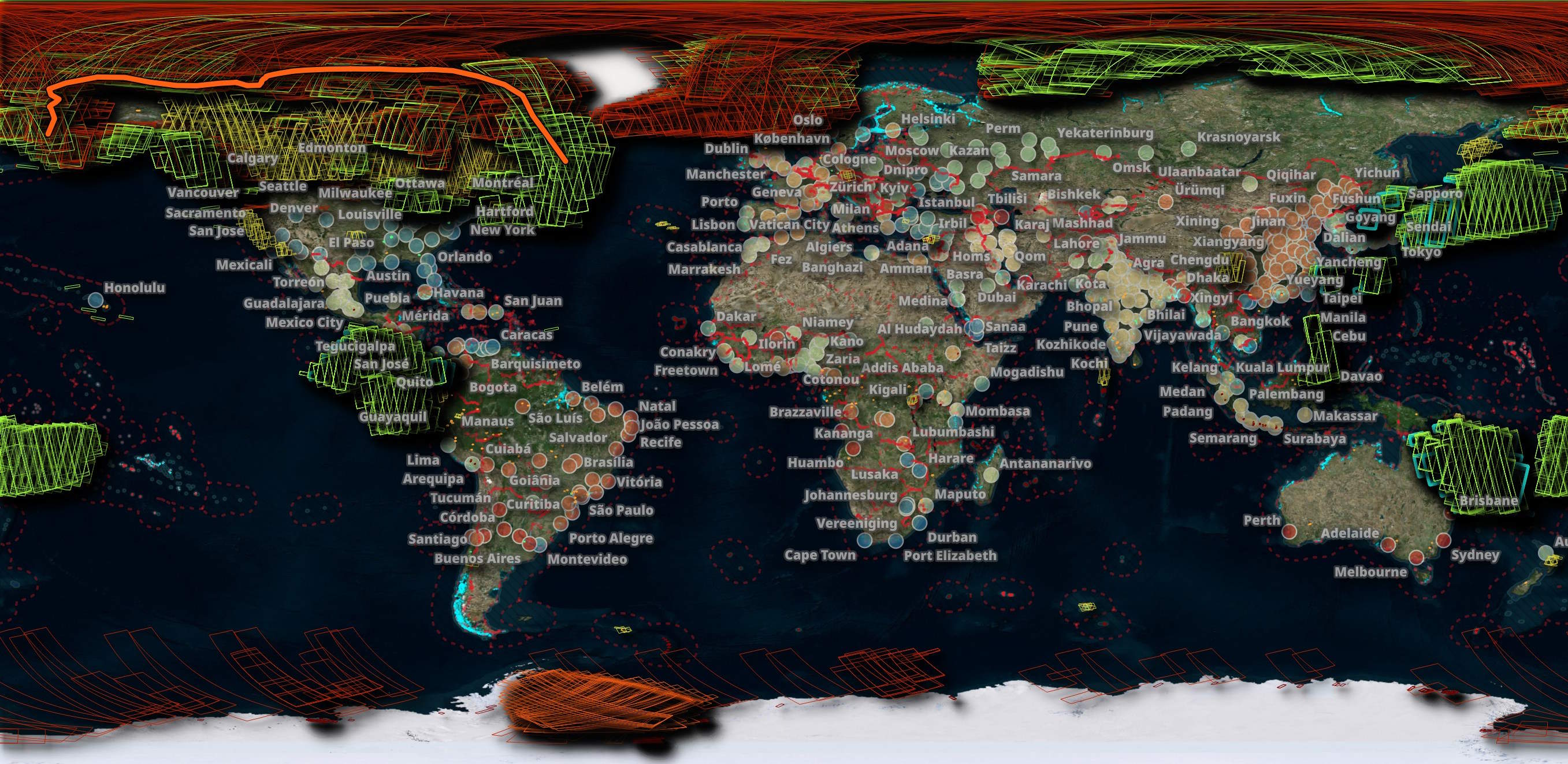
These are the footprint locations.
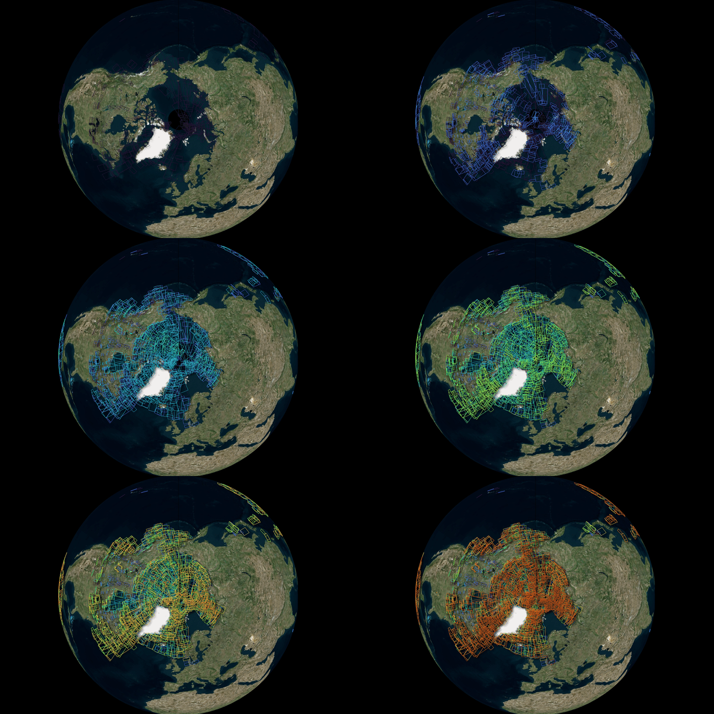
Below is an animation of part of the capture plan from earlier in the summer. I've coloured every footprint by its date and used the temporal functionality in QGIS to render them by the hour they were captured.
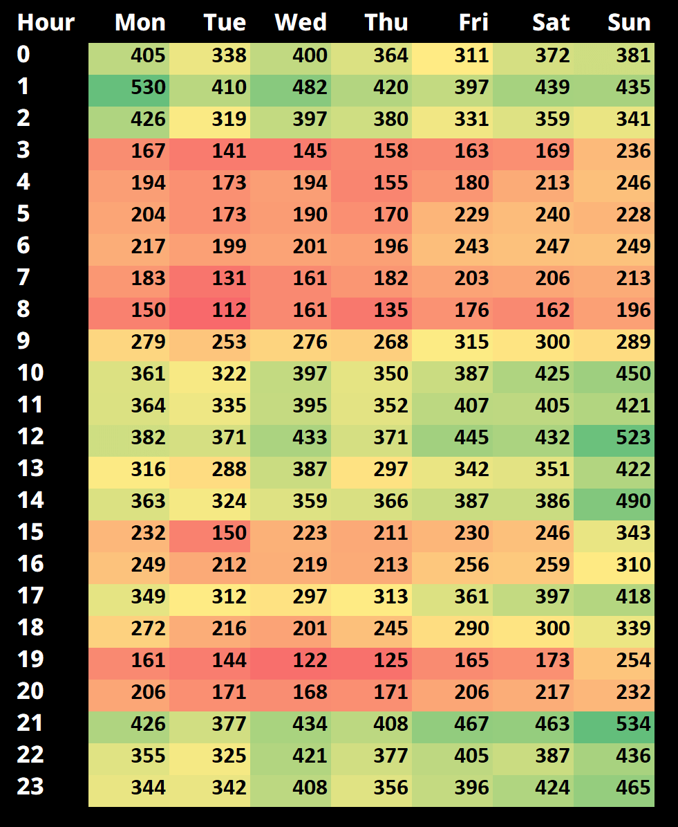
The capture times do have a relationship with the time of day in UTC and, to a lesser extent, the day of the week.
PIVOT    (
    SELECT   hour_:   HOUR(start_at),
             day_num: STRFTIME(start_at, '%u (%a)'),
             COUNT(*) cnt
    FROM     'RCM.parquet'
    GROUP BY 1, 2
)
ON       day_num
USING    SUM(cnt)
GROUP BY hour_
ORDER BY hour_;
Russia, Alaska & Fiji
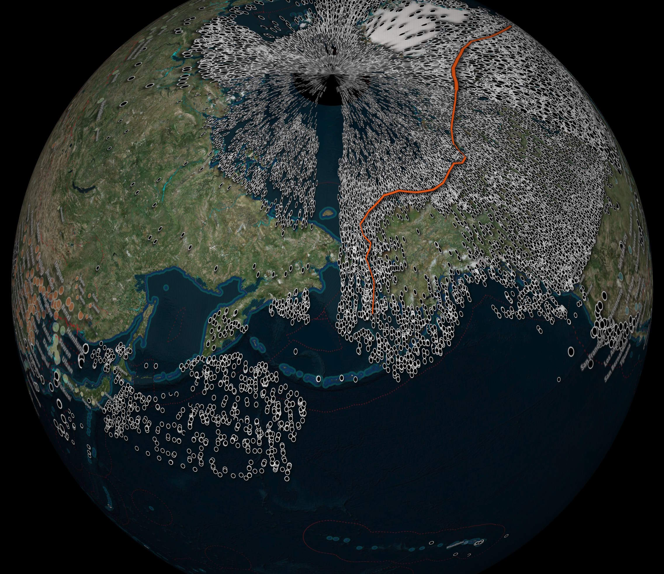
I noticed there are no footprint centroids that fall near -180W / 180E.
The South Pacific features heavily in the plans, but there are a lot of gaps around Fiji.
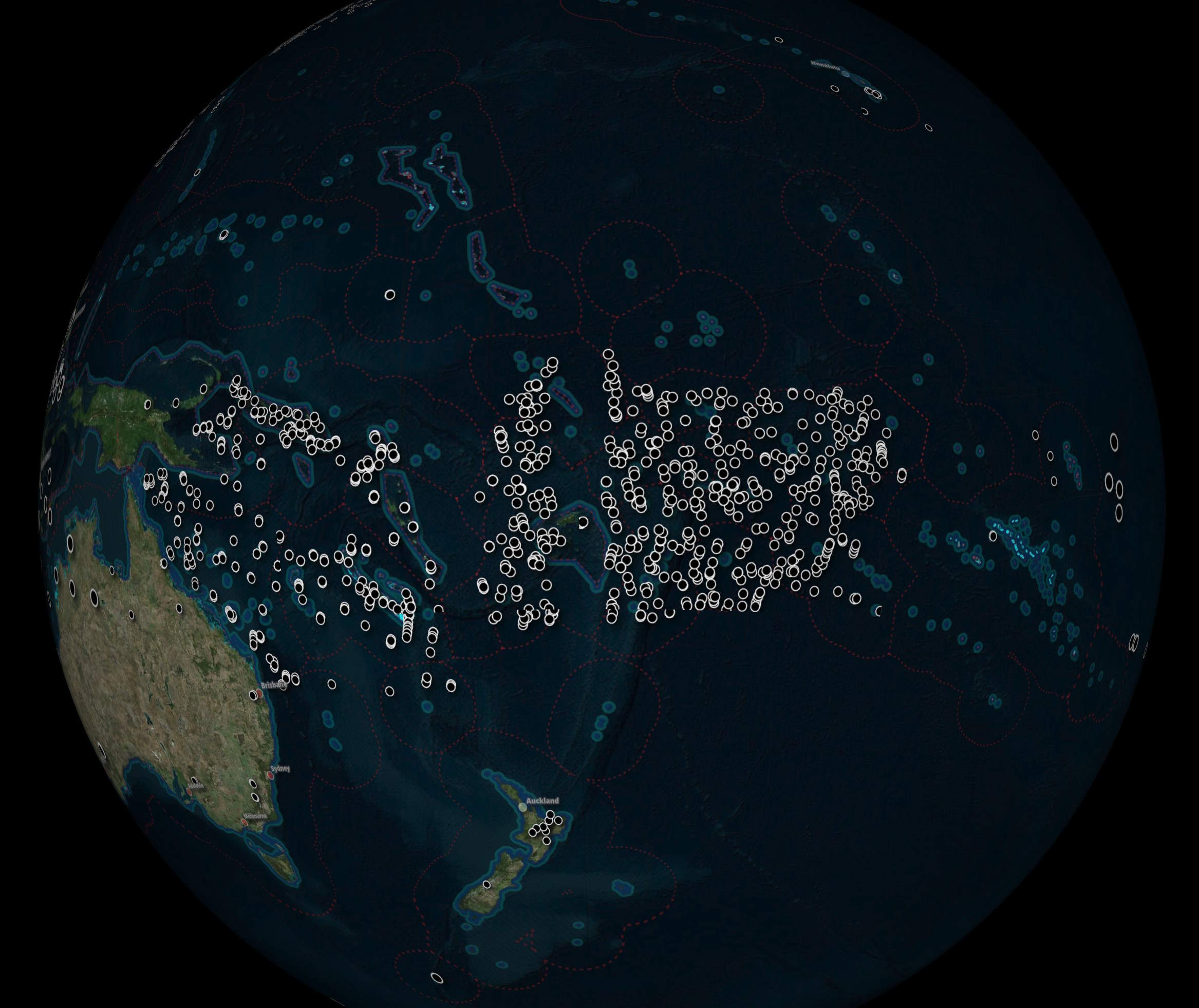
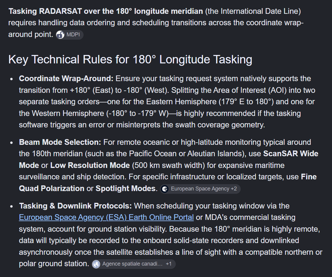
The vast footprint widths and heights supported mean these areas can still be captured, but either you can't task a footprint's centroid at this longitude, or there is some sort of plan-exporting issue.
The following is Google's take on RCM's longitude 180 support.
Local Capture Time
Given that SAR can see at night, I wondered if the local time of day played a major role in deciding when to capture any one area of interest (AOI).
I loaded Natural Earth's Time Zones dataset into DuckDB and excluded any zone associated with Antarctica (DuckDB's TIMEZONE function didn't accept any time zones from there).
$ ~/duckdb -nullvalue " "
CREATE OR REPLACE TABLE tz AS
    FROM  ST_READ('ne_10m_time_zones.shx')
    WHERE tz_name1st NOT LIKE 'Antarctica%';
I then joined each footprint centroid to its nearest time zone, converted the capture start time to the local time and counted how many footprints for each hour landed in each hexagon.
CREATE OR REPLACE TABLE hexagon_hours AS
    SELECT hexagon:         H3_LATLNG_TO_CELL(
                                ST_Y(ST_CENTROID(a.geometry)),
                                ST_X(ST_CENTROID(a.geometry)),
                                3),
           local_hour:      HOUR(TIMEZONE(tz_name1st, start_at)),
           num_footprints:  COUNT(*)
    FROM 'RCM.parquet' a
    JOIN tz ON tz.tz_name1st = (
        SELECT   tz.tz_name1st
        FROM     tz
        ORDER BY ST_DISTANCE(ST_Transform(
                                ST_CENTROID(a.geometry),
                                'OGC:CRS84',
                                'EPSG:4326'),
                             ST_CENTROID(tz.geom))
        LIMIT    1)
    GROUP BY 1, 2;
I then exported the most common local hour of capture for each hexagon.
COPY (
    SELECT geom: H3_CELL_TO_BOUNDARY_WKT(hexagon)::GEOMETRY,
           local_hour
    FROM (
        WITH b AS (
            SELECT *,
                   rn: ROW_NUMBER() OVER (PARTITION BY hexagon
                                          ORDER BY     num_footprints DESC)
            FROM   hexagon_hours
        )
        FROM     b
        WHERE    rn = 1
        ORDER BY num_footprints DESC
    )
    WHERE  ST_XMIN(H3_CELL_TO_BOUNDARY_WKT(hexagon)::geometry) BETWEEN -179 AND 179
    AND    ST_XMAX(H3_CELL_TO_BOUNDARY_WKT(hexagon)::geometry) BETWEEN -179 AND 179
    AND    ST_YMAX(H3_CELL_TO_BOUNDARY_WKT(hexagon)::geometry) BETWEEN -89  AND  89
) TO 'h3.local_hour.parquet' (
    FORMAT 'PARQUET',
    CODEC  'ZSTD',
    COMPRESSION_LEVEL 22,
    ROW_GROUP_SIZE 15000);
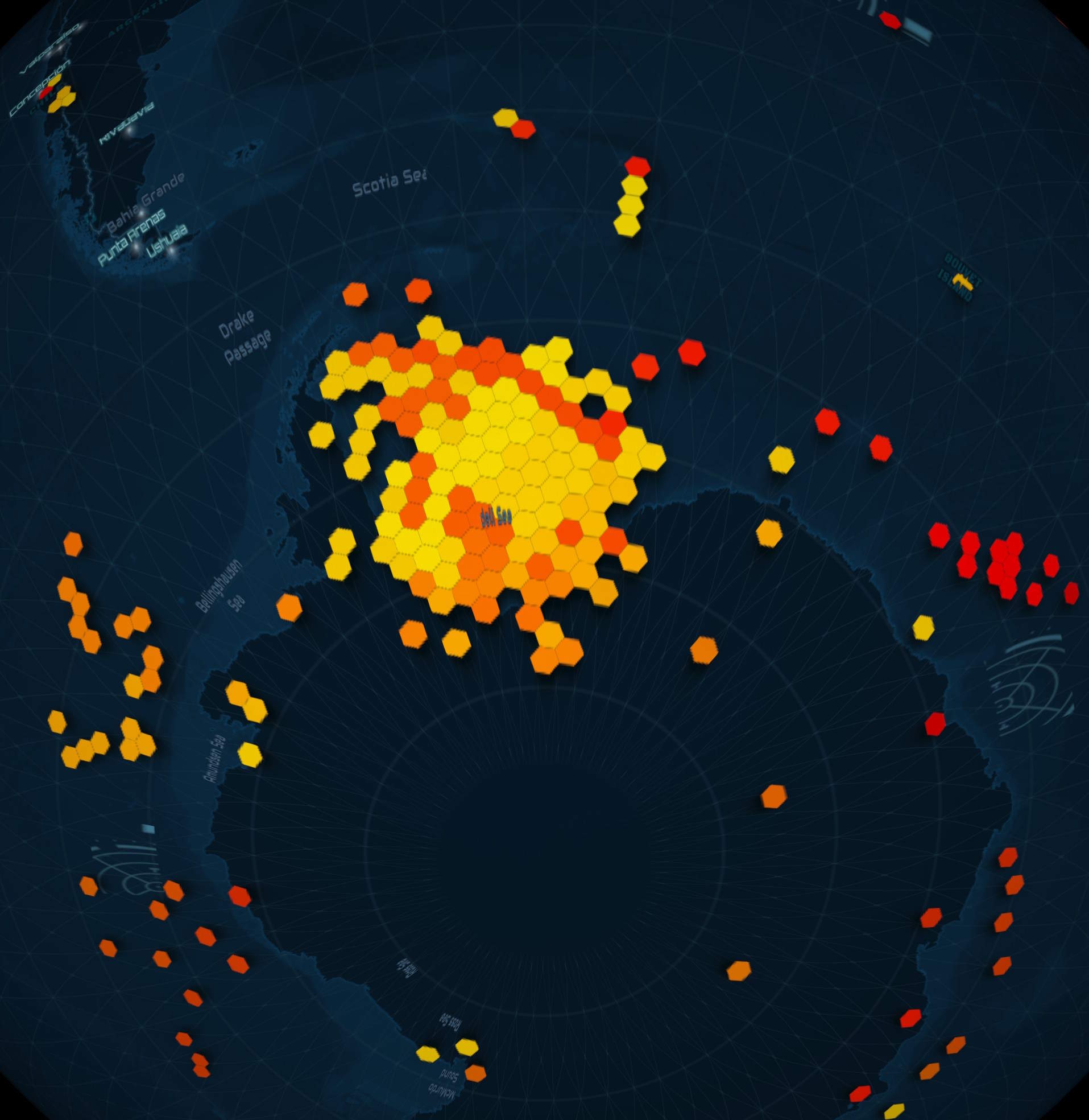
The yellow hexagons are at or closer to noon local time and red is at or closer to midnight.
With the exception of Greenland and Alaska, there doesn't appear to be a strong bias towards capturing at any particular local hour of the day.
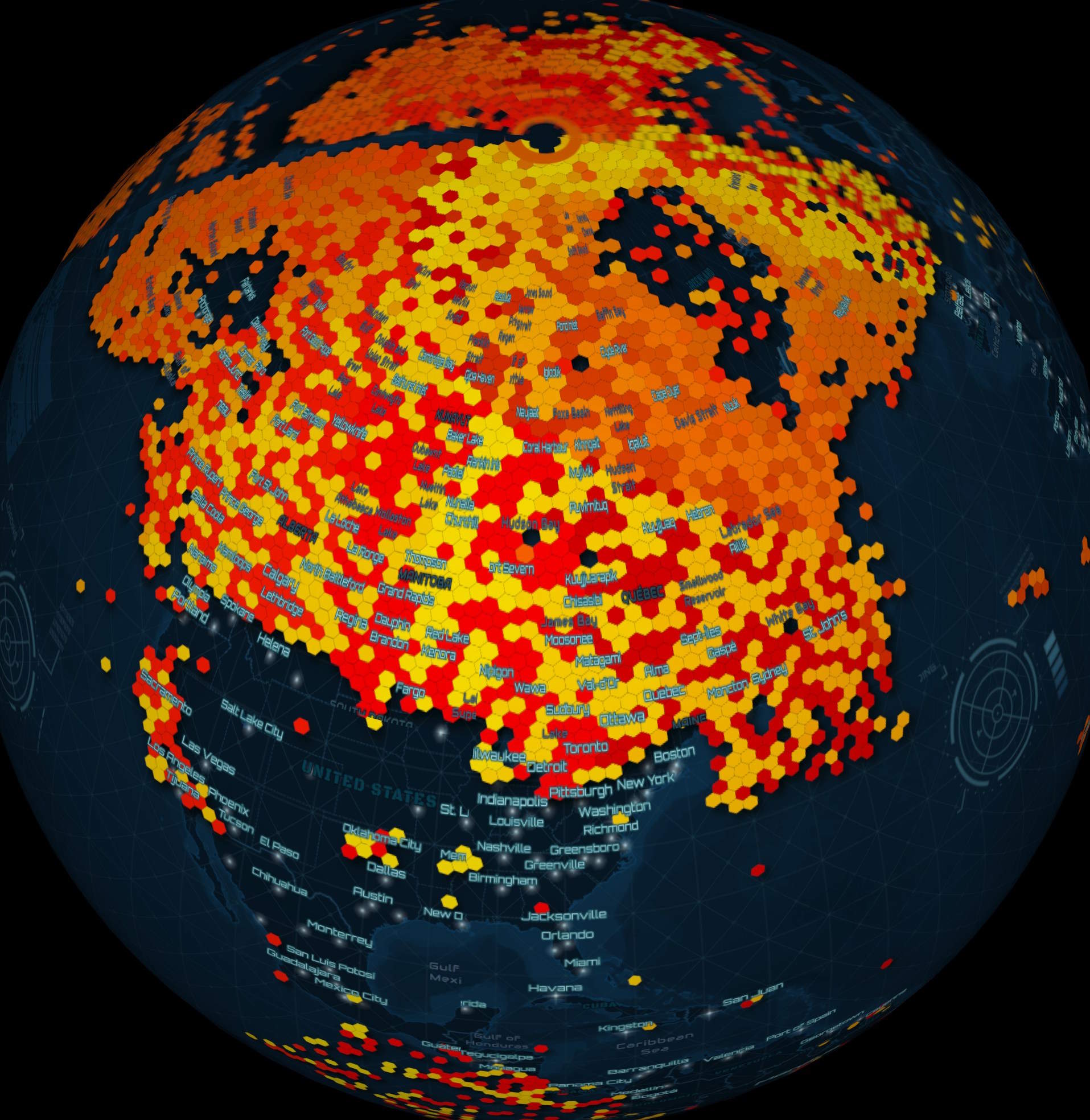
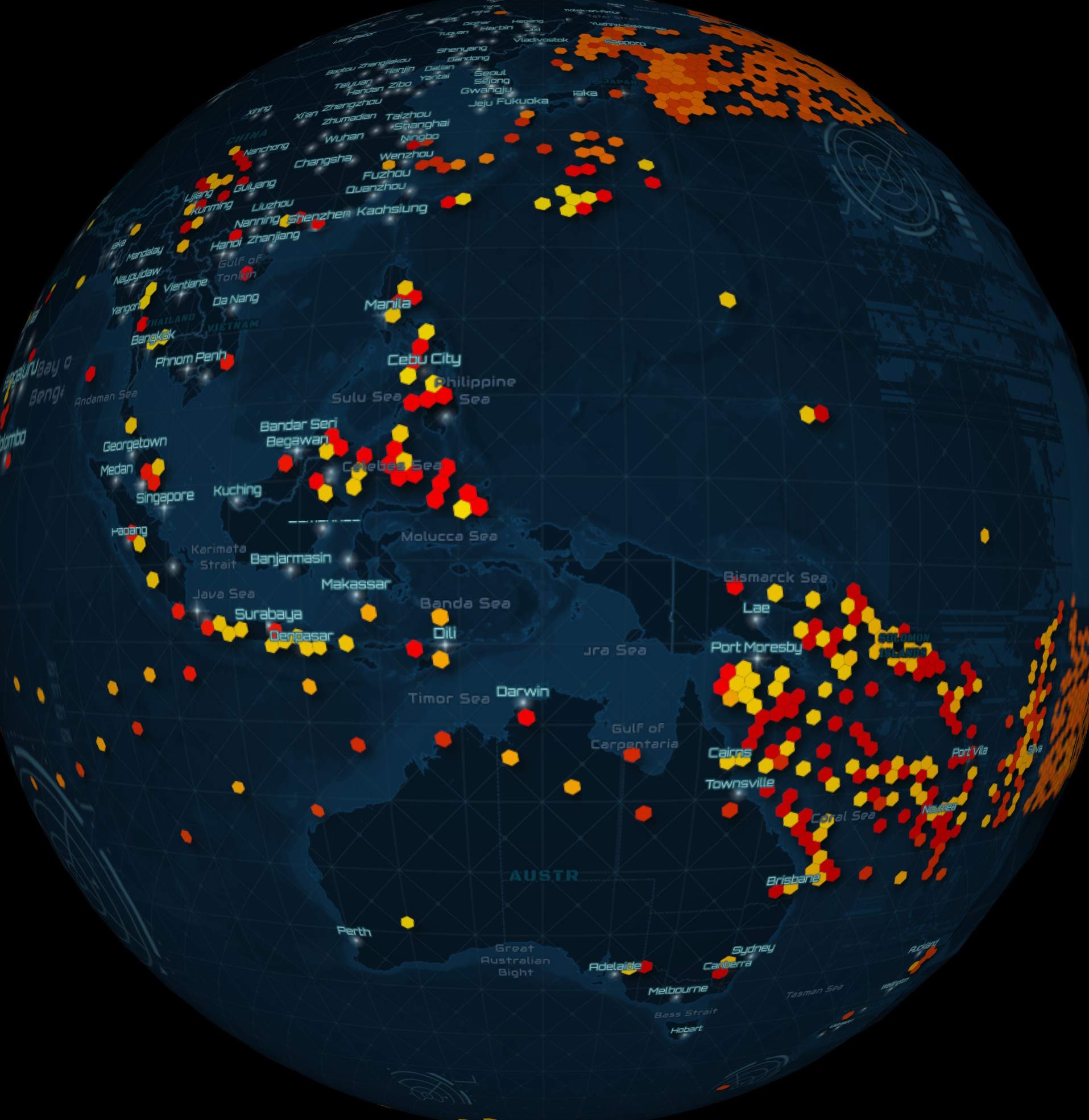
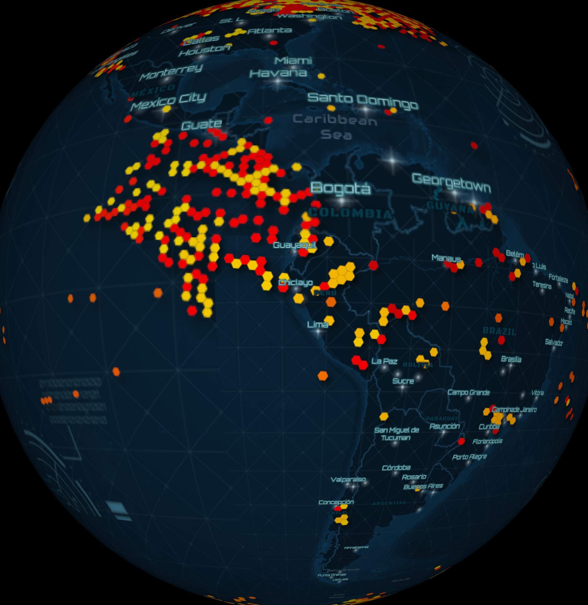
The closest I could find to a time-of-day bias is around Antarctica, where a previously-unknown Island was discovered recently. It might have been this imagery could be captured in a fairly narrow time frame. I'd have to examine RCM's TLEs to understand their orbits better.
Radar Modes & Beam Types
All the satellites in this constellation capture imagery across all beam types. The work appears to be spread evenly.
$ ~/duckdb -nullvalue " "
PIVOT (
    SELECT   sat_id,
             beam_type: REPLACE(beam_type, 'Resolution', 'R'),
             cnt:       COUNT(*)
    FROM     'RCM.parquet'
    GROUP BY 1, 2
    ORDER BY 1
)
ON       sat_id
USING    SUM(cnt)
GROUP BY beam_type
ORDER BY beam_type;
┌───────────────────┬────────┬────────┬────────┐
│     beam_type     │ RCM-1  │ RCM-2  │ RCM-3  │
│      varchar      │ int128 │ int128 │ int128 │
├───────────────────┼────────┼────────┼────────┤
│ High R 5m         │    580 │    581 │    611 │
│ Low Noise         │   6248 │   6281 │   6316 │
│ Low R 100m        │    805 │    784 │    624 │
│ Medium R 16m      │    277 │    271 │    282 │
│ Medium R 30m      │   2456 │   2475 │   2558 │
│ Medium R 50m      │   5923 │   5746 │   5723 │
│ Quad-Polarization │    111 │    102 │    104 │
│ Ship Detection    │    156 │    168 │    145 │
│ Spotlight         │    149 │     99 │    123 │
│ Very High R 3m    │    175 │    167 │    202 │
└───────────────────┴────────┴────────┴────────┘
The same goes for radar modes.
PIVOT (
    SELECT   sat_id,
             radar_md,
             cnt: COUNT(*)
    FROM     'RCM.parquet'
    GROUP BY 1, 2
    ORDER BY 1
)
ON       sat_id
USING    SUM(cnt)
GROUP BY radar_md
ORDER BY radar_md;
┌─────────────────────┬────────┬────────┬────────┐
│      radar_md       │ RCM-1  │ RCM-2  │ RCM-3  │
│       varchar       │ int128 │ int128 │ int128 │
├─────────────────────┼────────┼────────┼────────┤
│ ScanSAR             │  15588 │  15454 │  15366 │
│ Spotlight           │    149 │     99 │    123 │
│ Stripmap Continuous │   1143 │   1121 │   1199 │
└─────────────────────┴────────┴────────┴────────┘
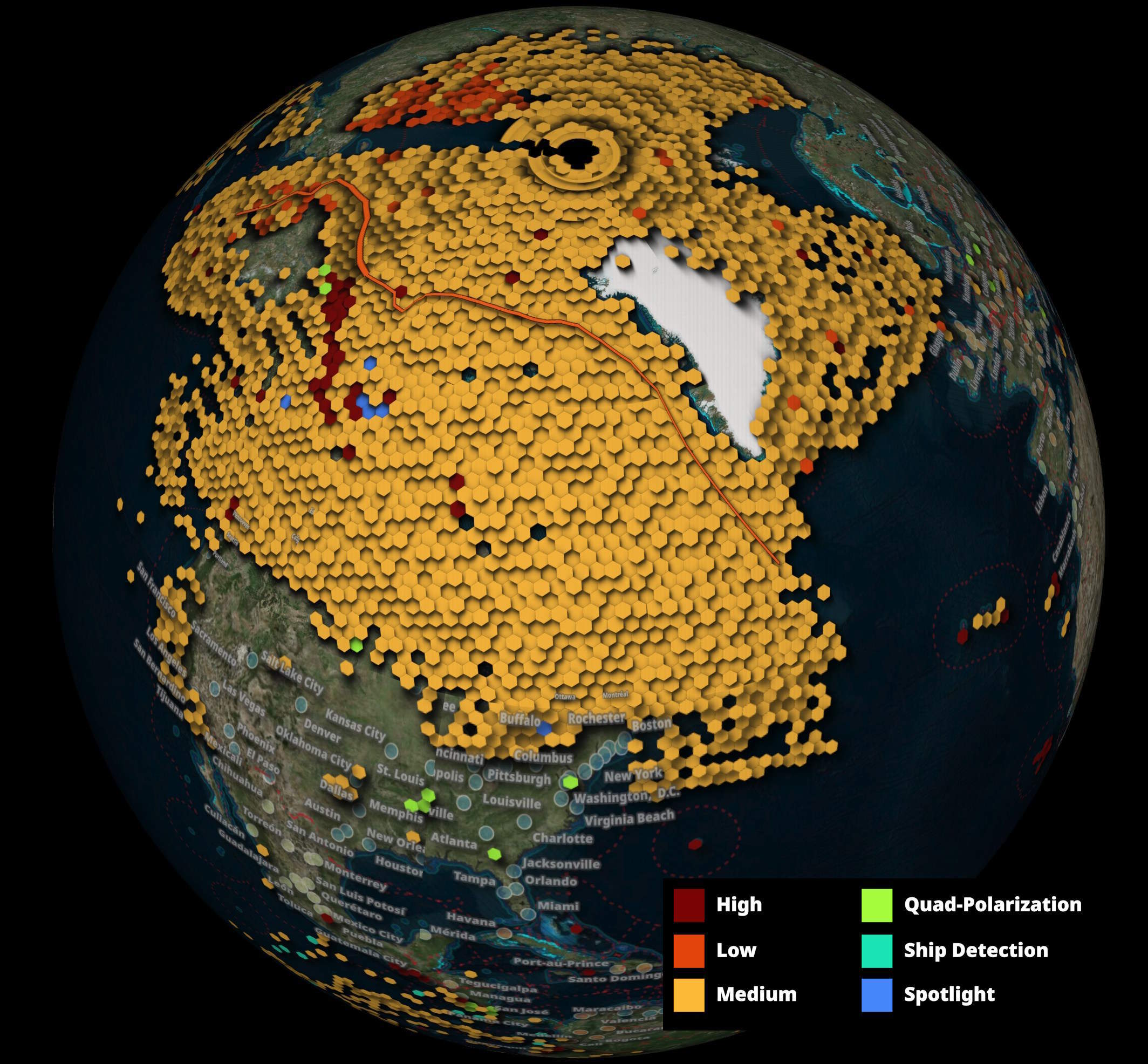
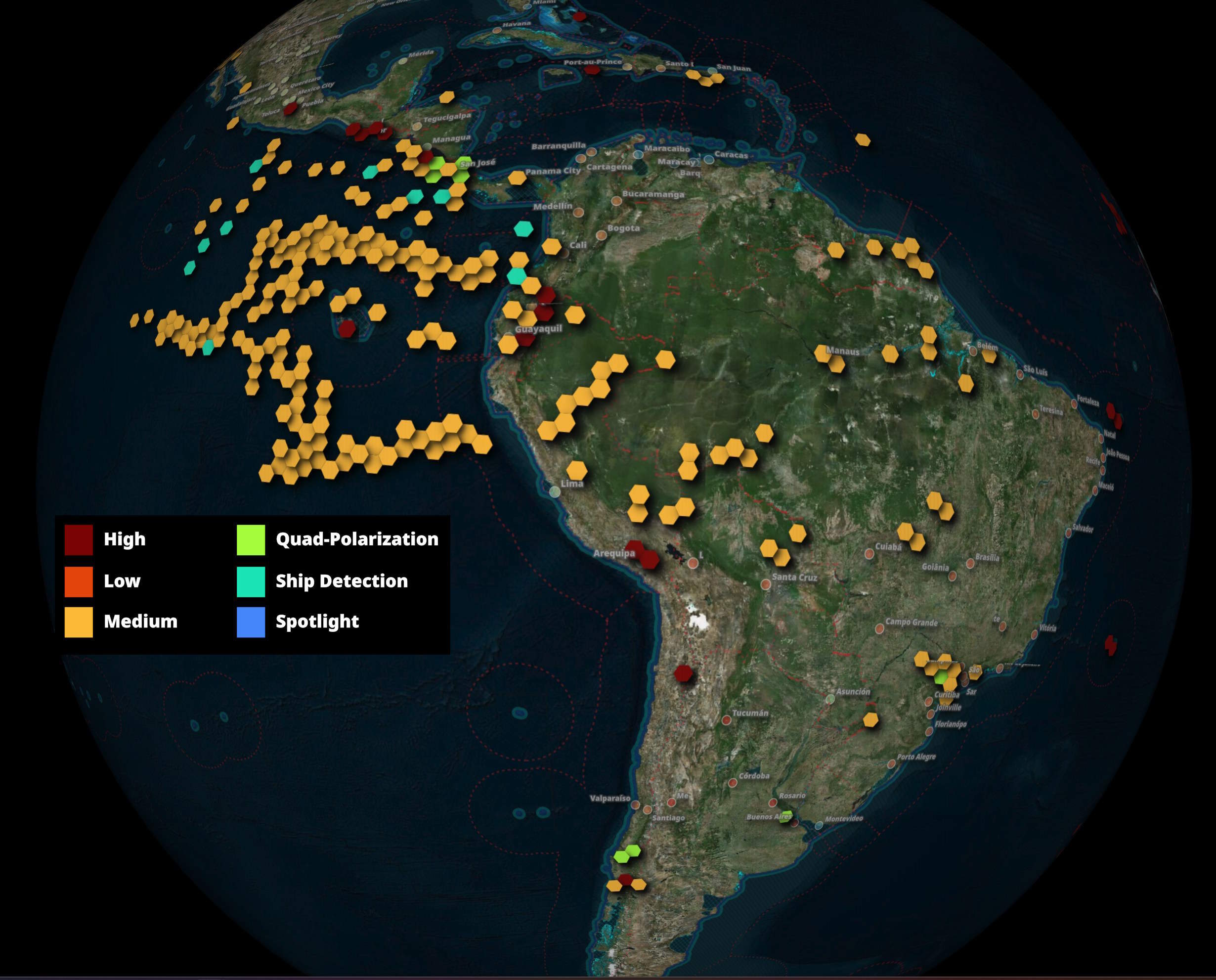
The "Very High R 3m", "Spotlight" and "Low Noise" beam types are often seen in high-latitude captures but don't appear as often below latitude 50. Ship detections are almost always below this latitude as well.
PIVOT (
    SELECT   below_50:  IF(ST_Y(ST_CENTROID(geometry)) <= 50, 'below', 'above'),
             beam_type: REPLACE(beam_type, 'Resolution', 'R'),
             cnt:       COUNT(*)
    FROM     'RCM.parquet'
    GROUP BY 1, 2
    ORDER BY 2
)
ON       below_50
USING    SUM(cnt)
GROUP BY beam_type
ORDER BY beam_type;
┌───────────────────┬────────┬────────┐
│     beam_type     │ above  │ below  │
│      varchar      │ int128 │ int128 │
├───────────────────┼────────┼────────┤
│ High R 5m         │   1047 │    725 │
│ Low Noise         │  18544 │    301 │
│ Low R 100m        │   1529 │    684 │
│ Medium R 16m      │    198 │    632 │
│ Medium R 30m      │   5334 │   2155 │
│ Medium R 50m      │  10937 │   6455 │
│ Quad-Polarization │    141 │    176 │
│ Ship Detection    │      8 │    461 │
│ Spotlight         │    262 │    109 │
│ Very High R 3m    │    493 │     51 │
└───────────────────┴────────┴────────┘
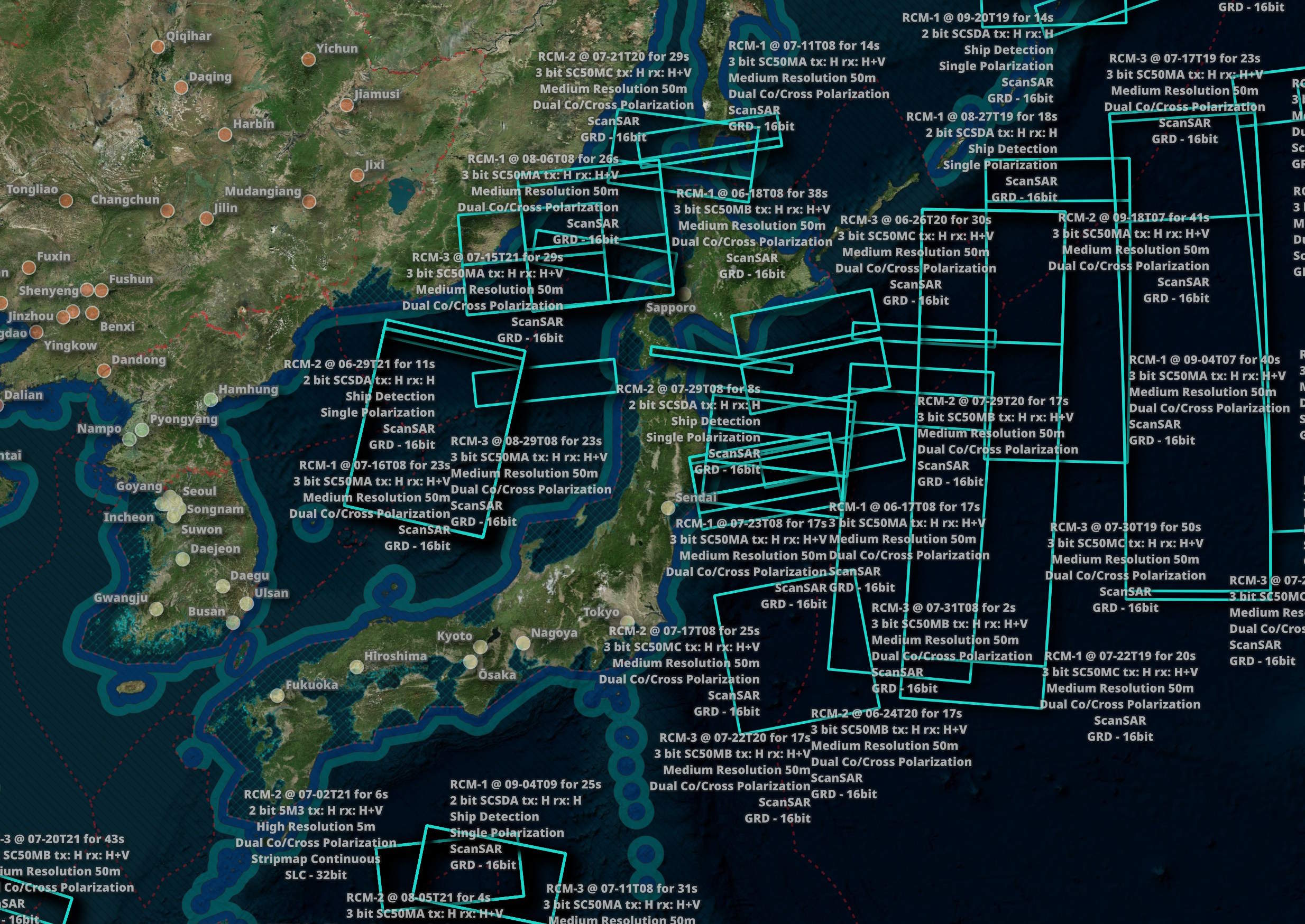
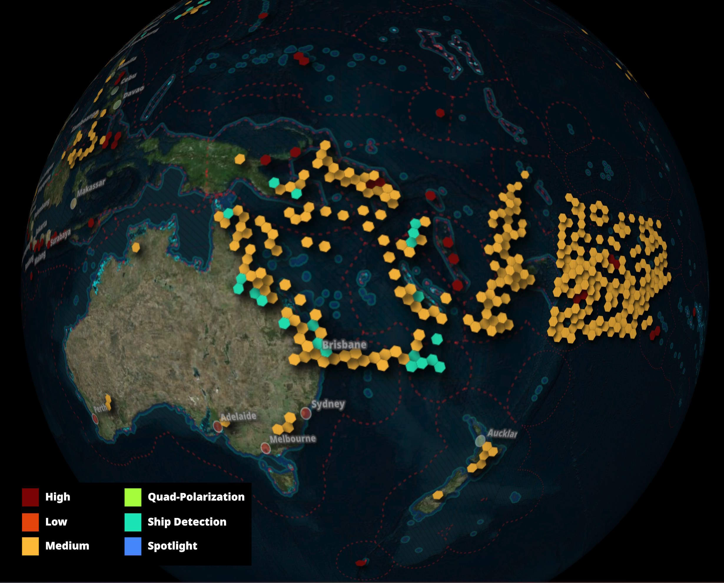
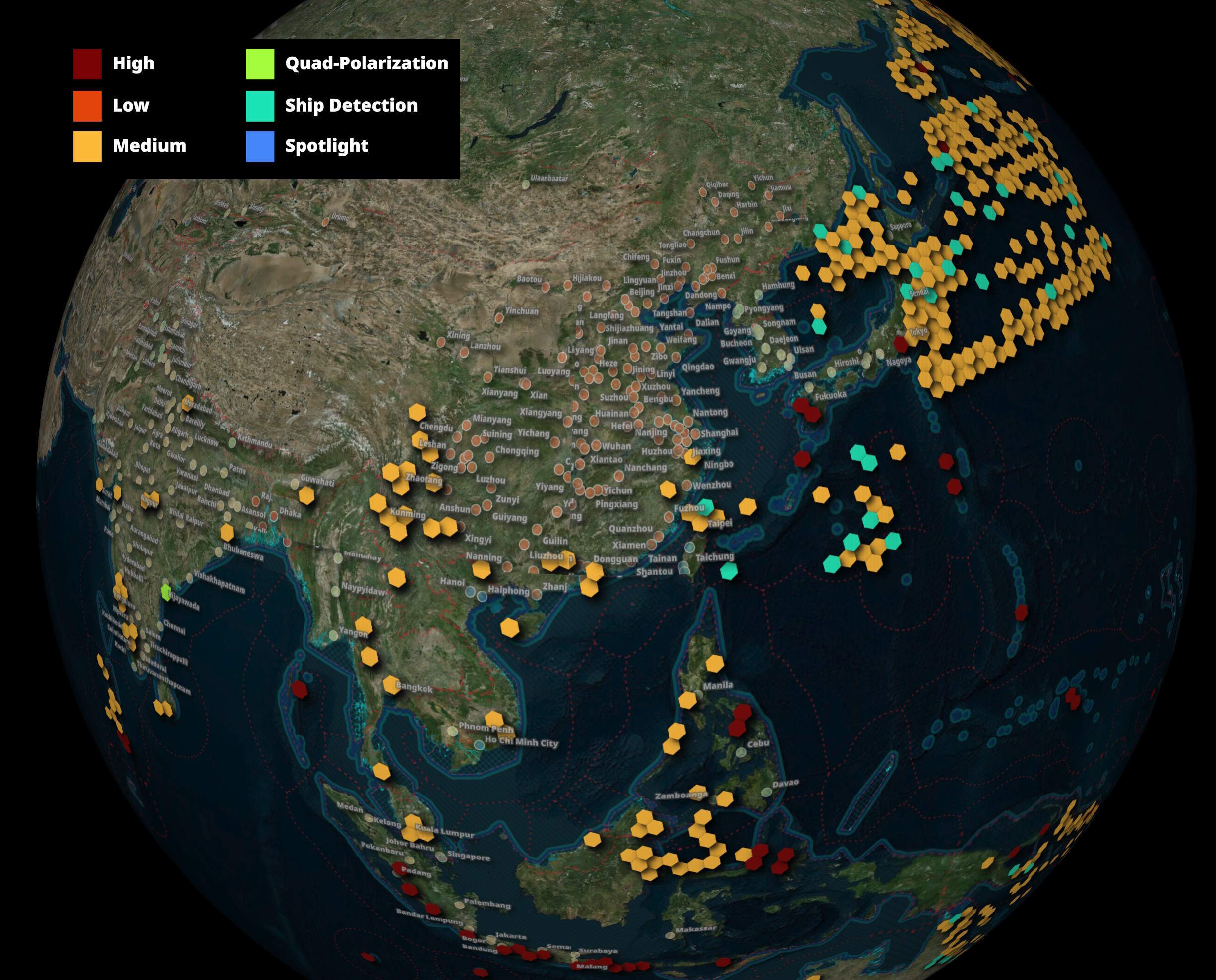
The light blue polygons represent the ship detection footprints.
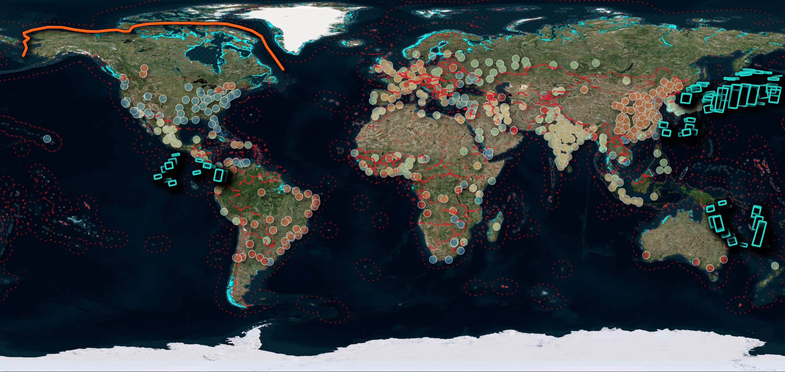
Below is a cluster of them around Japan.
The bulk of the ScanSAR radar mode happens above latitude 50.
PIVOT (
    SELECT   below_50: IF(ST_Y(ST_CENTROID(geometry)) <= 50, 'below', 'above'),
             radar_md,
             cnt: COUNT(*)
    FROM     'RCM.parquet'
    GROUP BY 1, 2
    ORDER BY 2
)
ON       below_50
USING    SUM(cnt)
GROUP BY radar_md
ORDER BY radar_md;
┌─────────────────────┬────────┬────────┐
│      radar_md       │ above  │ below  │
│       varchar       │ int128 │ int128 │
├─────────────────────┼────────┼────────┤
│ ScanSAR             │  36352 │  10056 │
│ Spotlight           │    262 │    109 │
│ Stripmap Continuous │   1879 │   1584 │
└─────────────────────┴────────┴────────┘
Duration is the only setting that changes for ship detection.
SELECT column_name,
       approx_unique,
       min,
       max
FROM   (SUMMARIZE
        FROM      'RCM.parquet'
        WHERE     beam_type = 'Ship Detection')
WHERE  column_name NOT IN ('geometry',
                           'bbox',
                           'start_at',
                           'end_at',
                           'uuid',
                           'longer_side',
                           'shorter_side');
┌──────────────────┬───────────────┬─────────────────────┬─────────────────────┐
│   column_name    │ approx_unique │         min         │         max         │
│     varchar      │     int64     │       varchar       │       varchar       │
├──────────────────┼───────────────┼─────────────────────┼─────────────────────┤
│ baq              │             1 │ 2 bit               │ 2 bit               │
│ beam_id          │             1 │ SCSDA               │ SCSDA               │
│ beam_type        │             1 │ Ship Detection      │ Ship Detection      │
│ ccd              │             1 │ false               │ false               │
│ ccd_exact        │             1 │ false               │ false               │
│ pol_type         │             1 │ Single Polarization │ Single Polarization │
│ prod_type        │             1 │ GRD - 16bit         │ GRD - 16bit         │
│ radar_md         │             1 │ ScanSAR             │ ScanSAR             │
│ rx_pol           │             1 │ H                   │ H                   │
│ sat_id           │             3 │ RCM-1               │ RCM-3               │
│ tx_pol           │             1 │ H                   │ H                   │
│ duration         │            49 │ 0                   │ 59                  │
│ simple_beam_type │             1 │ Ship Detection      │ Ship Detection      │
└──────────────────┴───────────────┴─────────────────────┴─────────────────────┘
Polarisation
Polarisation is very much based on the beam type.
$ ~/duckdb -nullvalue " "
PIVOT (
    SELECT   pol_type:  REPLACE(pol_type, 'Polarization', 'P.'),
             beam_type: REPLACE(beam_type, 'Resolution', 'R'),
             cnt:       COUNT(*)
    FROM     'RCM.parquet'
    GROUP BY 1, 2
    ORDER BY 1
)
ON       pol_type
USING    SUM(cnt)
GROUP BY beam_type
ORDER BY beam_type;
┌───────────────────┬────────────┬──────────────────┬───────────────┬─────────┬───────────┐
│     beam_type     │ Compact P. │ Dual Co/Cross P. │ Dual HH-VV P. │ Quad P. │ Single P. │
│      varchar      │   int128   │      int128      │    int128     │ int128  │  int128   │
├───────────────────┼────────────┼──────────────────┼───────────────┼─────────┼───────────┤
│ High R 5m         │        745 │              779 │               │         │       248 │
│ Low Noise         │        162 │            18683 │               │         │           │
│ Low R 100m        │            │              202 │          2011 │         │           │
│ Medium R 16m      │        707 │              123 │               │         │           │
│ Medium R 30m      │       6669 │              820 │               │         │           │
│ Medium R 50m      │         23 │            17355 │               │         │        14 │
│ Quad-Polarization │            │                  │               │     317 │           │
│ Ship Detection    │            │                  │               │         │       469 │
│ Spotlight         │         25 │                  │               │         │       346 │
│ Very High R 3m    │         11 │                1 │               │         │       532 │
└───────────────────┴────────────┴──────────────────┴───────────────┴─────────┴───────────┘
Coherent Change Detection (CCD) is only used for a handful of high-resolution modes. It'll likely be used to spot minute structural differences between two or more time-lapsed captures. RCM can revisit an exact ground path every four days, so CCD could be useful for spotting footprints and/or vehicle tire tracks before they fade.
PIVOT (
    SELECT   ccd:       IF(ccd, 'CCD', 'No CCD'),
             beam_type: REPLACE(beam_type, 'Resolution', 'R'),
             cnt:       COUNT(*)
    FROM     'RCM.parquet'
    GROUP BY 1, 2
    ORDER BY 1
)
ON       ccd
USING    SUM(cnt)
GROUP BY beam_type
ORDER BY beam_type;
┌───────────────────┬────────┬────────┐
│     beam_type     │  CCD   │ No CCD │
│      varchar      │ int128 │ int128 │
├───────────────────┼────────┼────────┤
│ High R 5m         │    442 │   1330 │
│ Low Noise         │        │  18845 │
│ Low R 100m        │        │   2213 │
│ Medium R 16m      │     62 │    768 │
│ Medium R 30m      │      5 │   7484 │
│ Medium R 50m      │        │  17392 │
│ Quad-Polarization │        │    317 │
│ Ship Detection    │        │    469 │
│ Spotlight         │    127 │    244 │
│ Very High R 3m    │    287 │    257 │
└───────────────────┴────────┴────────┘
The radar mode is tied to the beam type.
PIVOT (
    SELECT   radar_md,
             beam_type: REPLACE(beam_type, 'Resolution', 'R'),
             cnt:       COUNT(*)
    FROM     'RCM.parquet'
    GROUP BY 1, 2
    ORDER BY 1
)
ON       radar_md
USING    SUM(cnt)
GROUP BY beam_type
ORDER BY 2 DESC, 3 DESC, 4 DESC;
┌───────────────────┬─────────┬───────────┬─────────────────────┐
│     beam_type     │ ScanSAR │ Spotlight │ Stripmap Continuous │
│      varchar      │ int128  │  int128   │       int128        │
├───────────────────┼─────────┼───────────┼─────────────────────┤
│ Low Noise         │   18845 │           │                     │
│ Medium R 50m      │   17392 │           │                     │
│ Medium R 30m      │    7489 │           │                     │
│ Low R 100m        │    2213 │           │                     │
│ Ship Detection    │     469 │           │                     │
│ Spotlight         │         │       371 │                     │
│ High R 5m         │         │           │                1772 │
│ Medium R 16m      │         │           │                 830 │
│ Very High R 3m    │         │           │                 544 │
│ Quad-Polarization │         │           │                 317 │
└───────────────────┴─────────┴───────────┴─────────────────────┘
Most modes use cross-polarised horizontal (H) and vertical (V) reception polarisations. This is often used to measure volume scattering from vegetation canopies and structural roughness.
The horizontal radar polarisations are probably used for mapping sea ice, open water during windy conditions and double-bounce scattering from tree trunks or structures. The ship detection beam type uses this exclusively.
PIVOT (
    SELECT   rx_pol,
             beam_type: REPLACE(beam_type, 'Resolution', 'R'),
             cnt:       COUNT(*)
    FROM     'RCM.parquet'
    GROUP BY 1, 2
    ORDER BY 1
)
ON       rx_pol
USING    SUM(cnt)
GROUP BY beam_type
ORDER BY 3 DESC, 2 DESC;
┌───────────────────┬────────┬────────┐
│     beam_type     │   H    │  H+V   │
│      varchar      │ int128 │ int128 │
├───────────────────┼────────┼────────┤
│ Low Noise         │        │  18845 │
│ Medium R 50m      │     14 │  17378 │
│ Medium R 30m      │        │   7489 │
│ Low R 100m        │        │   2213 │
│ High R 5m         │    248 │   1524 │
│ Medium R 16m      │        │    830 │
│ Quad-Polarization │        │    317 │
│ Spotlight         │    346 │     25 │
│ Very High R 3m    │    532 │     12 │
│ Ship Detection    │    469 │        │
└───────────────────┴────────┴────────┘
These are the reception polarisations broken down by radar mode.
PIVOT (
    SELECT   rx_pol,
             radar_md,
             cnt: COUNT(*)
    FROM     'RCM.parquet'
    GROUP BY 1, 2
    ORDER BY 1
)
ON       rx_pol
USING    SUM(cnt)
GROUP BY radar_md
ORDER BY radar_md;
┌─────────────────────┬────────┬────────┐
│      radar_md       │   H    │  H+V   │
│       varchar       │ int128 │ int128 │
├─────────────────────┼────────┼────────┤
│ ScanSAR             │    483 │  45925 │
│ Spotlight           │    346 │     25 │
│ Stripmap Continuous │    780 │   2683 │
└─────────────────────┴────────┴────────┘
These are the transmission polarisations broken down by beam type.
PIVOT (
    SELECT   tx_pol,
             beam_type: REPLACE(beam_type, 'Resolution', 'R'),
             cnt:       COUNT(*)
    FROM     'RCM.parquet'
    GROUP BY 1, 2
    ORDER BY 1
)
ON       tx_pol
USING    SUM(cnt)
GROUP BY beam_type
ORDER BY 3 DESC;
┌───────────────────┬────────┬────────┬────────┬────────┐
│     beam_type     │   C    │   H    │  H+V   │   V    │
│      varchar      │ int128 │ int128 │ int128 │ int128 │
├───────────────────┼────────┼────────┼────────┼────────┤
│ Low Noise         │    162 │  18378 │        │    305 │
│ Medium R 50m      │     23 │  15409 │        │   1960 │
│ High R 5m         │    745 │   1027 │        │        │
│ Medium R 30m      │   6669 │    618 │        │    202 │
│ Very High R 3m    │     11 │    533 │        │        │
│ Ship Detection    │        │    469 │        │        │
│ Spotlight         │     25 │    346 │        │        │
│ Low R 100m        │        │    202 │   2011 │        │
│ Medium R 16m      │    707 │      6 │        │    117 │
│ Quad-Polarization │        │        │    317 │        │
└───────────────────┴────────┴────────┴────────┴────────┘
Beam Types
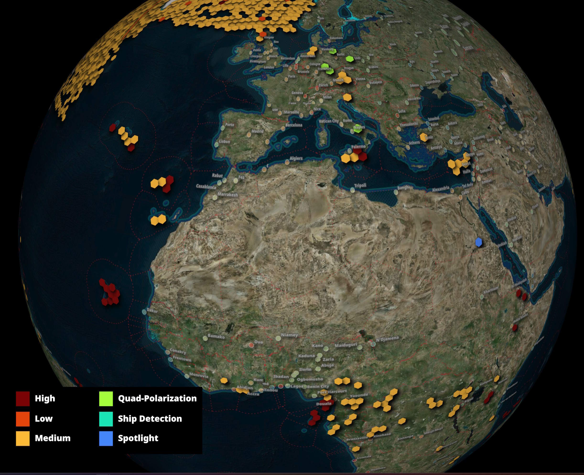
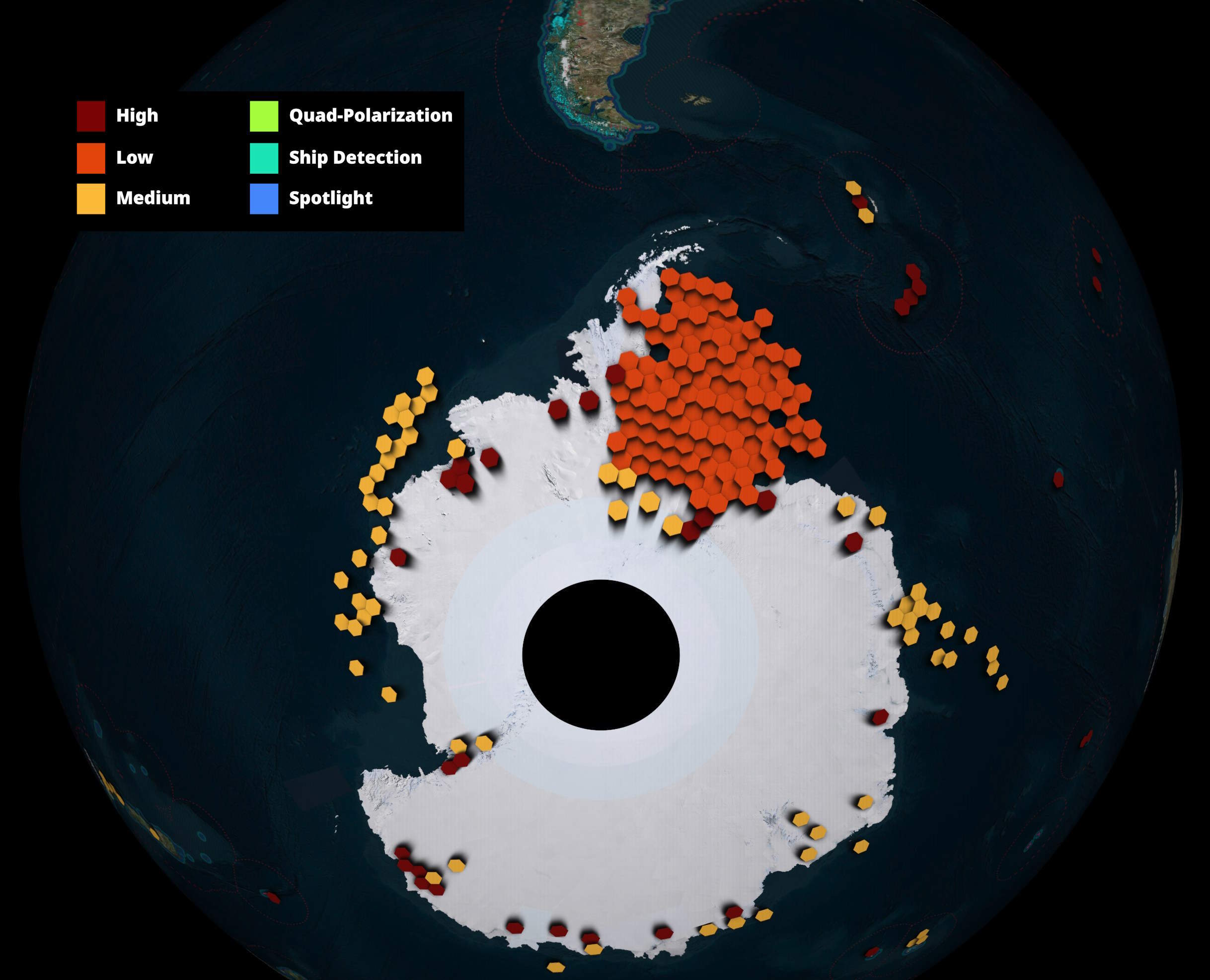
These are the most common beam types seen in RCM's plans.
$ ~/duckdb
COPY (
    SELECT geom: H3_CELL_TO_BOUNDARY_WKT(h3_3)::GEOMETRY,
           beam_type
    FROM   (
        WITH b AS (
                WITH a AS (
                    SELECT   h3_3: H3_LATLNG_TO_CELL(
                                        bbox.ymin,
                                        bbox.xmin,
                                        3) ,
                             beam_type:
                                CASE
                                WHEN beam_type ILIKE '%High%'   THEN 'High'
                                WHEN beam_type ILIKE '%Medium%' THEN 'Medium'
                                WHEN beam_type ILIKE '%Noise%'  THEN 'Medium'
                                WHEN beam_type ILIKE '%Low%'    THEN 'Low'
                                ELSE beam_type END,
                             num_recs: COUNT(*)
                    FROM     'RCM.parquet'
                    GROUP BY 1, 2
                )
                SELECT *,
                       rn: ROW_NUMBER() OVER (PARTITION BY h3_3
                                              ORDER BY     num_recs DESC)
                FROM   a
            )
            FROM     b
            WHERE    rn = 1
            ORDER BY num_recs DESC)
    WHERE  ST_XMIN(H3_CELL_TO_BOUNDARY_WKT(h3_3)::geometry) BETWEEN -179 AND 179
    AND    ST_XMAX(H3_CELL_TO_BOUNDARY_WKT(h3_3)::geometry) BETWEEN -179 AND 179
    AND    ST_YMAX(H3_CELL_TO_BOUNDARY_WKT(h3_3)::geometry) BETWEEN -89 AND 89
) TO 'h3_3.beam_type.parquet' (
    FORMAT 'PARQUET',
    CODEC  'ZSTD',
    COMPRESSION_LEVEL 22,
    ROW_GROUP_SIZE 15000);
Footprint Sizes
These are the footprint counts broken down by their width and height, measured in KMs.
$ ~/duckdb -nullvalue " "
PIVOT (
    SELECT   shorter: (ROUND(CEIL(shorter_side / 200000) * 200000) / 1000)::INT,
             longer:  (ROUND(CEIL(longer_side / 200000) * 200000) / 1000)::INT,
             cnt:     COUNT(*)
    FROM     'RCM.parquet'
    GROUP BY 1, 2
    ORDER BY 1, 2
)
ON       shorter IN (
            SELECT   DISTINCT shorter: (ROUND(CEIL(shorter_side / 200000) * 200000) / 1000)::INT
            FROM     'RCM.parquet'
            ORDER BY shorter::INT)
USING    SUM(cnt)
GROUP BY longer
ORDER BY longer;
┌────────┬────────┬────────┬────────┬────────┬────────┬────────┬────────┬────────┬────────┐
│ longer │  200   │  400   │  600   │  800   │  1000  │  1200  │  1400  │  1600  │  2000  │
│ int32  │ int128 │ int128 │ int128 │ int128 │ int128 │ int128 │ int128 │ int128 │ int128 │
├────────┼────────┼────────┼────────┼────────┼────────┼────────┼────────┼────────┼────────┤
│    200 │  10439 │        │        │        │        │        │        │        │        │
│    400 │  17925 │   3144 │        │        │        │        │        │        │        │
│    600 │   4714 │   7304 │   2075 │        │        │        │        │        │        │
│    800 │    194 │    895 │    791 │     38 │        │        │        │        │        │
│   1000 │     72 │    580 │    348 │     47 │        │        │        │        │        │
│   1200 │     31 │    291 │    259 │     32 │      8 │      1 │        │        │        │
│   1400 │     10 │    224 │    109 │     31 │     17 │      5 │      2 │        │        │
│   1600 │     17 │    114 │     64 │     23 │     33 │        │      1 │        │        │
│   1800 │      3 │     84 │     41 │      8 │     20 │        │        │        │        │
│   2000 │      7 │     46 │     24 │     19 │      4 │      8 │      2 │        │        │
│   2200 │      5 │     31 │      1 │      7 │      2 │     15 │      3 │      1 │        │
│   2400 │      1 │     31 │      4 │      6 │      1 │      3 │      2 │      4 │        │
│   2600 │      1 │      3 │        │      2 │        │      3 │      3 │        │      1 │
│   2800 │        │        │      2 │      1 │      1 │        │      2 │        │        │
│   3000 │        │        │        │        │      2 │        │        │        │        │
└────────┴────────┴────────┴────────┴────────┴────────┴────────┴────────┴────────┴────────┘
These are the beam type counts for the nearest 200 KMs of the longer side of each footprint.
PIVOT (
    SELECT   beam_type:   REPLACE(beam_type, 'Resolution', 'R'),
             longer_side: (ROUND(CEIL(longer_side / 200000) * 200000) / 1000)::INT,
             cnt:         COUNT(*)
    FROM     'RCM.parquet'
    GROUP BY 1, 2
) ON     longer_side IN (
            SELECT   DISTINCT longer_side: (ROUND(CEIL(longer_side / 200000) * 200000) / 1000)::INT
            FROM     'RCM.parquet'
            ORDER BY longer_side::INT)
USING    SUM(cnt)
GROUP BY beam_type
ORDER BY beam_type;
┌───────────────────┬────────┬────────┬────────┬────────┬────────┬────────┬────────┬────────┬────────┬────────┬────────┬────────┬────────┬────────┬────────┐
│     beam_type     │  200   │  400   │  600   │  800   │  1000  │  1200  │  1400  │  1600  │  1800  │  2000  │  2200  │  2400  │  2600  │  2800  │  3000  │
│      varchar      │ int128 │ int128 │ int128 │ int128 │ int128 │ int128 │ int128 │ int128 │ int128 │ int128 │ int128 │ int128 │ int128 │ int128 │ int128 │
├───────────────────┼────────┼────────┼────────┼────────┼────────┼────────┼────────┼────────┼────────┼────────┼────────┼────────┼────────┼────────┼────────┤
│ High R 5m         │   1749 │     20 │      3 │        │        │        │        │        │        │        │        │        │        │        │        │
│ Low Noise         │    270 │   9556 │   7956 │    493 │    221 │    115 │     63 │     54 │     35 │     29 │     27 │     11 │      9 │      4 │      2 │
│ Low R 100m        │     61 │   1215 │    435 │    210 │    100 │     83 │     55 │     44 │      8 │      2 │        │        │        │        │        │
│ Medium R 16m      │    830 │        │        │        │        │        │        │        │        │        │        │        │        │        │        │
│ Medium R 30m      │   6072 │    880 │    308 │    132 │     44 │     27 │      5 │     11 │      2 │      6 │      2 │        │        │        │        │
│ Medium R 50m      │    226 │   9018 │   5356 │   1052 │    674 │    388 │    268 │    143 │    111 │     73 │     36 │     41 │      4 │      2 │        │
│ Quad-Polarization │    316 │      1 │        │        │        │        │        │        │        │        │        │        │        │        │        │
│ Ship Detection    │        │    379 │     35 │     31 │      8 │      9 │      7 │        │        │        │        │        │        │        │        │
│ Spotlight         │    371 │        │        │        │        │        │        │        │        │        │        │        │        │        │        │
│ Very High R 3m    │    544 │        │        │        │        │        │        │        │        │        │        │        │        │        │        │
└───────────────────┴────────┴────────┴────────┴────────┴────────┴────────┴────────┴────────┴────────┴────────┴────────┴────────┴────────┴────────┴────────┘
These are the reception polarisations counts broken down by the shorter side of each footprint, rounded to the nearest 200 KMs.
PIVOT  (
    SELECT   rx_pol,
             shorter_side: (ROUND(CEIL(shorter_side / 200000) * 200000) / 1000)::INT,
             cnt:          COUNT(*)
    FROM     'RCM.parquet'
    WHERE    shorter_side > 0
    GROUP BY 1, 2
)
ON       rx_pol
USING    SUM(cnt)
GROUP BY shorter_side
ORDER BY shorter_side;
┌──────────────┬────────┬────────┐
│ shorter_side │   H    │  H+V   │
│    int32     │ int128 │ int128 │
├──────────────┼────────┼────────┤
│          200 │   1383 │  32036 │
│          400 │    226 │  12521 │
│          600 │        │   3718 │
│          800 │        │    214 │
│         1000 │        │     88 │
│         1200 │        │     35 │
│         1400 │        │     15 │
│         1600 │        │      5 │
│         2000 │        │      1 │
└──────────────┴────────┴────────┘
These are the transmission polarisations counts broken down by the shorter side of each footprint, rounded to the nearest 200 KMs.
PIVOT (
    SELECT   tx_pol,
             shorter_side: (ROUND(CEIL(shorter_side / 200000) * 200000) / 1000)::INT,
             cnt:          COUNT(*)
    FROM     'RCM.parquet'
    WHERE    shorter_side > 0
    GROUP BY 1, 2
)
ON       tx_pol
USING    SUM(cnt)
GROUP BY shorter_side
ORDER BY shorter_side;
┌──────────────┬────────┬────────┬────────┬────────┐
│ shorter_side │   C    │   H    │  H+V   │   V    │
│    int32     │ int128 │ int128 │ int128 │ int128 │
├──────────────┼────────┼────────┼────────┼────────┤
│          200 │   8258 │  22105 │   1328 │   1728 │
│          400 │     69 │  11151 │    742 │    785 │
│          600 │     11 │   3419 │    217 │     71 │
│          800 │      3 │    182 │     29 │        │
│         1000 │      1 │     79 │      8 │        │
│         1200 │        │     34 │      1 │        │
│         1400 │        │     12 │      3 │        │
│         1600 │        │      5 │        │        │
│         2000 │        │      1 │        │        │
└──────────────┴────────┴────────┴────────┴────────┘
These are the reception polarisations counts broken down by the longer side of each footprint, rounded to the nearest 200 KMs.
PIVOT (
    SELECT   rx_pol,
             longer_side: (ROUND(CEIL(longer_side / 200000) * 200000) / 1000)::INT,
             cnt:         COUNT(*)
    FROM     'RCM.parquet'
    WHERE    longer_side > 0
    GROUP BY 1, 2
)
ON       rx_pol
USING    SUM(cnt)
GROUP BY longer_side
ORDER BY longer_side;
┌─────────────┬────────┬────────┐
│ longer_side │   H    │  H+V   │
│    int32    │ int128 │ int128 │
├─────────────┼────────┼────────┤
│         200 │   1126 │   9313 │
│         400 │    388 │  20681 │
│         600 │     40 │  14053 │
│         800 │     31 │   1887 │
│        1000 │      8 │   1039 │
│        1200 │      9 │    613 │
│        1400 │      7 │    391 │
│        1600 │        │    252 │
│        1800 │        │    156 │
│        2000 │        │    110 │
│        2200 │        │     65 │
│        2400 │        │     52 │
│        2600 │        │     13 │
│        2800 │        │      6 │
│        3000 │        │      2 │
└─────────────┴────────┴────────┘
These are the transmission polarisations counts broken down by the longer side of each footprint, rounded to the nearest 200 KMs.
PIVOT (
    SELECT   tx_pol,
             longer_side: (ROUND(CEIL(longer_side / 200000) * 200000) / 1000)::INT,
             cnt:         COUNT(*)
    FROM     'RCM.parquet'
    GROUP BY 1, 2
)
ON       tx_pol
USING    SUM(cnt)
GROUP BY longer_side
ORDER BY longer_side;
┌─────────────┬────────┬────────┬────────┬────────┐
│ longer_side │   C    │   H    │  H+V   │   V    │
│    int32    │ int128 │ int128 │ int128 │ int128 │
├─────────────┼────────┼────────┼────────┼────────┤
│         200 │   6879 │   2867 │    377 │    316 │
│         400 │    853 │  17038 │   1216 │   1962 │
│         600 │    380 │  13182 │    307 │    224 │
│         800 │    127 │   1599 │    137 │     55 │
│        1000 │     47 │    879 │     99 │     22 │
│        1200 │     28 │    506 │     83 │      5 │
│        1400 │      7 │    336 │     55 │        │
│        1600 │     11 │    197 │     44 │        │
│        1800 │      2 │    146 │      8 │        │
│        2000 │      6 │    102 │      2 │        │
│        2200 │      2 │     63 │        │        │
│        2400 │        │     52 │        │        │
│        2600 │        │     13 │        │        │
│        2800 │        │      6 │        │        │
│        3000 │        │      2 │        │        │
└─────────────┴────────┴────────┴────────┴────────┘
These are the footprint counts for each of the receiving and transmission polarisation pairs.
PIVOT (
    SELECT   tx_pol,
             rx_pol,
             cnt: COUNT(*)
    FROM     'RCM.parquet'
    GROUP BY 1, 2
)
ON       rx_pol
USING    SUM(cnt)
GROUP BY tx_pol
ORDER BY tx_pol;
┌─────────┬────────┬────────┐
│ tx_pol  │   H    │  H+V   │
│ varchar │ int128 │ int128 │
├─────────┼────────┼────────┤
│ C       │        │   8342 │
│ H       │   1609 │  35379 │
│ H+V     │        │   2328 │
│ V       │        │   2584 │
└─────────┴────────┴────────┘
These are the polarisation type counts broken down by the shorter side of each footprint, rounded to the nearest 200 KMs.
PIVOT (
    SELECT   pol_type,
             shorter_side: (ROUND(CEIL(shorter_side / 200000) * 200000) / 1000)::INT,
             cnt:          COUNT(*)
    FROM     'RCM.parquet'
    GROUP BY 1, 2
)
ON       shorter_side IN (
            SELECT   DISTINCT shorter_side: (ROUND(CEIL(shorter_side / 200000) * 200000) / 1000)::INT
            FROM     'RCM.parquet'
            ORDER BY shorter_side::INT)
USING    SUM(cnt)
GROUP BY pol_type
ORDER BY pol_type;
┌────────────────────────────┬────────┬────────┬────────┬────────┬────────┬────────┬────────┬────────┬────────┐
│          pol_type          │  200   │  400   │  600   │  800   │  1000  │  1200  │  1400  │  1600  │  2000  │
│          varchar           │ int128 │ int128 │ int128 │ int128 │ int128 │ int128 │ int128 │ int128 │ int128 │
├────────────────────────────┼────────┼────────┼────────┼────────┼────────┼────────┼────────┼────────┼────────┤
│ Compact Polarization       │   8258 │     69 │     11 │      3 │      1 │        │        │        │        │
│ Dual Co/Cross Polarization │  22450 │  11710 │   3490 │    182 │     79 │     34 │     12 │      5 │      1 │
│ Dual HH-VV Polarization    │   1011 │    742 │    217 │     29 │      8 │      1 │      3 │        │        │
│ Quad Polarization          │    317 │        │        │        │        │        │        │        │        │
│ Single Polarization        │   1383 │    226 │        │        │        │        │        │        │        │
└────────────────────────────┴────────┴────────┴────────┴────────┴────────┴────────┴────────┴────────┴────────┘
These are the polarisation type counts broken down by the longer side of each footprint, rounded to the nearest 200 KMs.
PIVOT (
    SELECT   pol_type,
             longer_side: (ROUND(CEIL(longer_side / 200000) * 200000) / 1000)::INT,
             cnt:         COUNT(*)
    FROM     'RCM.parquet'
    GROUP BY 1, 2
)
ON       longer_side IN (
            SELECT   DISTINCT longer_side: (ROUND(CEIL(longer_side / 200000) * 200000) / 1000)::INT
            FROM     'RCM.parquet'
            ORDER BY longer_side::INT)
USING    SUM(cnt)
GROUP BY pol_type
ORDER BY pol_type;
┌────────────────────────────┬────────┬────────┬────────┬────────┬────────┬────────┬────────┬────────┬────────┬────────┬────────┬────────┬────────┬────────┬────────┐
│          pol_type          │  200   │  400   │  600   │  800   │  1000  │  1200  │  1400  │  1600  │  1800  │  2000  │  2200  │  2400  │  2600  │  2800  │  3000  │
│          varchar           │ int128 │ int128 │ int128 │ int128 │ int128 │ int128 │ int128 │ int128 │ int128 │ int128 │ int128 │ int128 │ int128 │ int128 │ int128 │
├────────────────────────────┼────────┼────────┼────────┼────────┼────────┼────────┼────────┼────────┼────────┼────────┼────────┼────────┼────────┼────────┼────────┤
│ Compact Polarization       │   6879 │    853 │    380 │    127 │     47 │     28 │      7 │     11 │      2 │      6 │      2 │        │        │        │        │
│ Dual Co/Cross Polarization │   2057 │  18612 │  13366 │   1623 │    893 │    502 │    329 │    197 │    146 │    102 │     63 │     52 │     13 │      6 │      2 │
│ Dual HH-VV Polarization    │     61 │   1215 │    307 │    137 │     99 │     83 │     55 │     44 │      8 │      2 │        │        │        │        │        │
│ Quad Polarization          │    316 │      1 │        │        │        │        │        │        │        │        │        │        │        │        │        │
│ Single Polarization        │   1126 │    388 │     40 │     31 │      8 │      9 │      7 │        │        │        │        │        │        │        │        │
└────────────────────────────┴────────┴────────┴────────┴────────┴────────┴────────┴────────┴────────┴────────┴────────┴────────┴────────┴────────┴────────┴────────┘
These are the number of captures each satellite will make, broken down by the shorter side of each footprint, rounded to the nearest 200 KMs.
PIVOT (
    SELECT   sat_id,
             shorter_side: (ROUND(CEIL(shorter_side / 200000) * 200000) / 1000)::INT,
             cnt:          COUNT(*)
    FROM     'RCM.parquet'
    GROUP BY 1, 2
)
ON       sat_id
USING    SUM(cnt)
GROUP BY shorter_side
ORDER BY shorter_side;
┌──────────────┬────────┬────────┬────────┐
│ shorter_side │ RCM-1  │ RCM-2  │ RCM-3  │
│    int32     │ int128 │ int128 │ int128 │
├──────────────┼────────┼────────┼────────┤
│          200 │  11255 │  11030 │  11134 │
│          400 │   4357 │   4272 │   4118 │
│          600 │   1149 │   1272 │   1297 │
│          800 │     79 │     62 │     73 │
│         1000 │     32 │     16 │     40 │
│         1200 │      5 │     15 │     15 │
│         1400 │      2 │      5 │      8 │
│         1600 │      1 │      2 │      2 │
│         2000 │        │        │      1 │
└──────────────┴────────┴────────┴────────┘
These are the number of captures each satellite will make, broken down by the longer side of each footprint, rounded to the nearest 200 KMs.
PIVOT (
    SELECT   sat_id,
             longer_side: (ROUND(CEIL(shorter_side / 200000) * 200000) / 1000)::INT,
             cnt:         COUNT(*)
    FROM     'RCM.parquet'
    GROUP BY 1, 2
)
ON       sat_id
USING    SUM(cnt)
GROUP BY longer_side
ORDER BY longer_side;
┌─────────────┬────────┬────────┬────────┐
│ longer_side │ RCM-1  │ RCM-2  │ RCM-3  │
│    int32    │ int128 │ int128 │ int128 │
├─────────────┼────────┼────────┼────────┤
│         200 │  11255 │  11030 │  11134 │
│         400 │   4357 │   4272 │   4118 │
│         600 │   1149 │   1272 │   1297 │
│         800 │     79 │     62 │     73 │
│        1000 │     32 │     16 │     40 │
│        1200 │      5 │     15 │     15 │
│        1400 │      2 │      5 │      8 │
│        1600 │      1 │      2 │      2 │
│        2000 │        │        │      1 │
└─────────────┴────────┴────────┴────────┘
Capture Durations
These are the capture lengths rounded to the next six seconds for each beam type. Three of these modes don't have any documented examples of capturing imagery longer than 30 seconds, and Spotlight is likely under six seconds max.
$ ~/duckdb -nullvalue " "
PIVOT (
    SELECT   duration:  (CEIL(duration / 6) * 6)::INT,
             beam_type: REPLACE(beam_type, 'Resolution', 'R'),
             cnt:       COUNT(*)
    FROM     'RCM.parquet'
    GROUP BY 1, 2
    ORDER BY 1
)
ON duration IN (
            SELECT   DISTINCT (CEIL(duration / 6) * 6)::INT
            FROM     'RCM.parquet'
            ORDER BY (CEIL(duration / 6) * 6)::INT)
USING    SUM(cnt)
GROUP BY beam_type
ORDER BY 12 DESC;
┌───────────────────┬────────┬────────┬────────┬────────┬────────┬────────┬────────┬────────┬────────┬────────┬────────┐
│     beam_type     │   0    │   6    │   12   │   18   │   24   │   30   │   36   │   42   │   48   │   54   │   60   │
│      varchar      │ int128 │ int128 │ int128 │ int128 │ int128 │ int128 │ int128 │ int128 │ int128 │ int128 │ int128 │
├───────────────────┼────────┼────────┼────────┼────────┼────────┼────────┼────────┼────────┼────────┼────────┼────────┤
│ Medium R 50m      │     56 │   1028 │   2201 │   4214 │   2179 │   1812 │   1730 │   1292 │   1223 │    936 │    721 │
│ Low Noise         │     14 │    561 │   2271 │   6871 │   2684 │   1916 │   1550 │   1044 │    801 │    632 │    501 │
│ Low R 100m        │        │     65 │     67 │    798 │    290 │    247 │    222 │    198 │    132 │     98 │     96 │
│ Medium R 30m      │     17 │   1577 │   2232 │   1283 │    827 │    522 │    370 │    269 │    199 │    127 │     66 │
│ Ship Detection    │      2 │     16 │     50 │     72 │     56 │    101 │     32 │     32 │     76 │     27 │      5 │
│ High R 5m         │        │    869 │    590 │    229 │     56 │     13 │     10 │      2 │      1 │      1 │      1 │
│ Quad-Polarization │        │    276 │     32 │      4 │      3 │      1 │        │      1 │        │        │        │
│ Medium R 16m      │        │    699 │    116 │      9 │      6 │        │        │        │        │        │        │
│ Very High R 3m    │        │    270 │    258 │     14 │      2 │        │        │        │        │        │        │
│ Spotlight         │        │    371 │        │        │        │        │        │        │        │        │        │
└───────────────────┴────────┴────────┴────────┴────────┴────────┴────────┴────────┴────────┴────────┴────────┴────────┘
These are the durations rounded up to the next three seconds for each radar mode.
PIVOT (
    SELECT   duration: (CEIL(duration / 3) * 3)::INT,
             radar_md,
             cnt: COUNT(*)
    FROM     'RCM.parquet'
    GROUP BY 1, 2
    ORDER BY 1
)
ON       radar_md
USING    SUM(cnt)
GROUP BY duration
ORDER BY duration;
┌──────────┬─────────┬───────────┬─────────────────────┐
│ duration │ ScanSAR │ Spotlight │ Stripmap Continuous │
│  int32   │ int128  │  int128   │       int128        │
├──────────┼─────────┼───────────┼─────────────────────┤
│        0 │      89 │           │                     │
│        3 │     678 │       295 │                 239 │
│        6 │    2569 │        76 │                1875 │
│        9 │    2328 │           │                 806 │
│       12 │    4493 │           │                 190 │
│       15 │    3667 │           │                 194 │
│       18 │    9571 │           │                  62 │
│       21 │    3240 │           │                  48 │
│       24 │    2796 │           │                  19 │
│       27 │    2398 │           │                   8 │
│       30 │    2200 │           │                   6 │
│       33 │    2094 │           │                   5 │
│       36 │    1810 │           │                   5 │
│       39 │    1552 │           │                   1 │
│       42 │    1283 │           │                   2 │
│       45 │    1311 │           │                   1 │
│       48 │    1120 │           │                     │
│       51 │    1054 │           │                     │
│       54 │     766 │           │                   1 │
│       57 │     770 │           │                   1 │
│       60 │     619 │           │                     │
└──────────┴─────────┴───────────┴─────────────────────┘
All capture durations are possible at all footprint widths and lengths. There is no limitation that longer captures are only available for shorter distances until the beam type is factored in.
PIVOT (
    SELECT   duration:     (CEIL(duration / 10) * 10)::INT,
             shorter_side: (ROUND(CEIL(shorter_side / 200000) * 200000) / 1000)::INT,
             cnt:          COUNT(*)
    FROM     'RCM.parquet'
    GROUP BY 1, 2
)
ON       duration
USING    SUM(cnt)
GROUP BY shorter_side
ORDER BY shorter_side;
┌──────────────┬────────┬────────┬────────┬────────┬────────┬────────┬────────┐
│ shorter_side │   0    │   10   │   20   │   30   │   40   │   50   │   60   │
│    int32     │ int128 │ int128 │ int128 │ int128 │ int128 │ int128 │ int128 │
├──────────────┼────────┼────────┼────────┼────────┼────────┼────────┼────────┤
│          200 │     16 │   7678 │  18141 │   6056 │    860 │    446 │    222 │
│          400 │     30 │    745 │   1157 │   1385 │   4475 │   3484 │   1471 │
│          600 │     43 │   1073 │    887 │    459 │    353 │    354 │    549 │
│          800 │        │     36 │     35 │     30 │     27 │     53 │     33 │
│         1000 │        │     12 │     21 │     16 │     14 │     13 │     12 │
│         1200 │        │      7 │      3 │      6 │      3 │      5 │     11 │
│         1400 │        │      2 │      6 │      1 │      3 │      1 │      2 │
│         1600 │        │      1 │        │        │      2 │      1 │      1 │
│         2000 │        │        │      1 │        │        │        │        │
└──────────────┴────────┴────────┴────────┴────────┴────────┴────────┴────────┘
PIVOT (
    SELECT   duration:    (CEIL(duration / 10) * 10)::INT,
             longer_side: (ROUND(CEIL(longer_side / 200000) * 200000) / 1000)::INT,
             cnt:         COUNT(*)
    FROM     'RCM.parquet'
    GROUP BY 1, 2
)
ON       duration
USING    SUM(cnt)
GROUP BY longer_side
ORDER BY longer_side;
┌─────────────┬────────┬────────┬────────┬────────┬────────┬────────┬────────┐
│ longer_side │   0    │   10   │   20   │   30   │   40   │   50   │   60   │
│    int32    │ int128 │ int128 │ int128 │ int128 │ int128 │ int128 │ int128 │
├─────────────┼────────┼────────┼────────┼────────┼────────┼────────┼────────┤
│         200 │        │   6273 │   3021 │   1130 │     15 │        │        │
│         400 │      1 │   1224 │  12206 │   3526 │   2375 │   1407 │    330 │
│         600 │     57 │   1342 │   4433 │   2515 │   2444 │   1981 │   1321 │
│         800 │      1 │     84 │    133 │    421 │    557 │    596 │    126 │
│        1000 │     17 │    387 │    169 │     74 │     50 │     75 │    275 │
│        1200 │        │     42 │     86 │    138 │    154 │    157 │     45 │
│        1400 │     11 │     99 │     86 │     20 │     29 │     35 │    118 │
│        1600 │        │      8 │     30 │     74 │     67 │     50 │     23 │
│        1800 │      2 │     65 │     13 │     10 │      7 │     22 │     37 │
│        2000 │        │      4 │     25 │     30 │     24 │     21 │      6 │
│        2200 │        │     20 │     23 │      4 │      1 │      4 │     13 │
│        2400 │        │      3 │     23 │      4 │     12 │      4 │      6 │
│        2600 │        │        │      3 │      6 │      1 │      3 │        │
│        2800 │        │      2 │        │        │      1 │      2 │      1 │
│        3000 │        │      1 │        │      1 │        │        │        │
└─────────────┴────────┴────────┴────────┴────────┴────────┴────────┴────────┘
Deliverables
Single Look Complex (SLC) is the native, highest-resolution Level-1 SAR product. It preserves both the amplitude (brightness) and phase (distance to the target) information. This product is good for classifying surface materials.
Multi-Look Complex (MLC) can deliver imagery with less background noise and speckle. This can be good for measuring ocean waves.
Ground Range Detected (GRD) is often used for regular mapping, land cover classification, ship detection and disaster monitoring.
The following are the numbers of GRD, MLC and SLC deliverables broken down by beam type.
$ ~/duckdb -nullvalue " "
PIVOT (
    SELECT   prod_type: SPLIT(prod_type, ' -')[1],
             beam_type: REPLACE(beam_type, 'Resolution', 'R'),
             cnt:       COUNT(*)
    FROM     'RCM.parquet'
    GROUP BY 1, 2
    ORDER BY 1
)
ON       prod_type
USING    SUM(cnt)
GROUP BY beam_type
ORDER BY 2 DESC;
┌───────────────────┬────────┬────────┬────────┬────────┐
│     beam_type     │  GRD   │  MLC   │  SLC   │  null  │
│      varchar      │ int128 │ int128 │ int128 │ int128 │
├───────────────────┼────────┼────────┼────────┼────────┤
│ Low Noise         │  18683 │    162 │        │        │
│ Medium R 50m      │  17369 │     23 │        │        │
│ Low R 100m        │   2213 │        │        │        │
│ Ship Detection    │    469 │        │        │        │
│ Medium R 30m      │    338 │   5825 │   1198 │    128 │
│ High R 5m         │    156 │        │   1292 │    324 │
│ Medium R 16m      │    118 │        │    712 │        │
│ Very High R 3m    │      1 │        │    543 │        │
│ Spotlight         │        │        │    371 │        │
│ Quad-Polarization │        │        │    317 │        │
└───────────────────┴────────┴────────┴────────┴────────┘
The following are the numbers of GRD, MLC and SLC deliverables broken down by radar mode.
PIVOT (
    SELECT   prod_type: SPLIT(prod_type, ' -')[1],
             radar_md,
             cnt: COUNT(*)
    FROM     'RCM.parquet'
    GROUP BY 1, 2
    ORDER BY 1
)
ON       prod_type
USING    SUM(cnt)
GROUP BY radar_md
ORDER BY 2 DESC;
┌─────────────────────┬────────┬────────┬────────┬────────┐
│      radar_md       │  GRD   │  MLC   │  SLC   │  null  │
│       varchar       │ int128 │ int128 │ int128 │ int128 │
├─────────────────────┼────────┼────────┼────────┼────────┤
│ ScanSAR             │  39072 │   6010 │   1198 │    128 │
│ Stripmap Continuous │    275 │        │   2864 │    324 │
│ Spotlight           │        │        │    371 │        │
└─────────────────────┴────────┴────────┴────────┴────────┘
This is the 16- and 32-bit deliverable breakdown by radar mode.
PIVOT (
    SELECT   prod_type: SPLIT(prod_type, ' - ')[2],
             radar_md,
             cnt: COUNT(*)
    FROM     'RCM.parquet'
    GROUP BY 1, 2
    ORDER BY 1
)
ON       prod_type
USING    SUM(cnt)
GROUP BY radar_md
ORDER BY 2 DESC;
┌─────────────────────┬────────┬────────┐
│      radar_md       │ 16bit  │ 32bit  │
│       varchar       │ int128 │ int128 │
├─────────────────────┼────────┼────────┤
│ ScanSAR             │  41255 │   5153 │
│ Stripmap Continuous │    989 │   2474 │
│ Spotlight           │     95 │    276 │
└─────────────────────┴────────┴────────┘
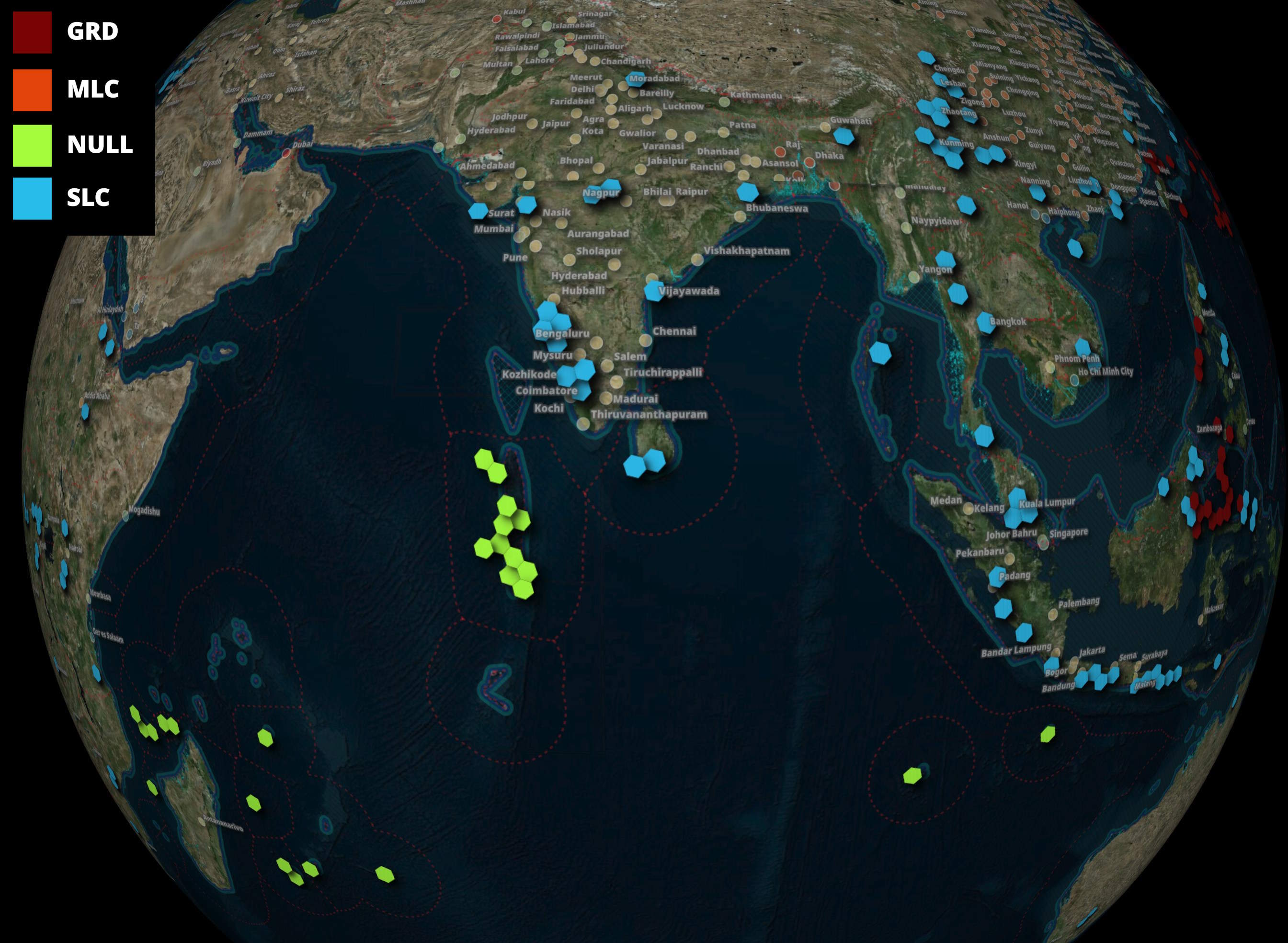
There does seem to be a relationship between location and most common deliverable.
COPY (
    SELECT geom: H3_CELL_TO_BOUNDARY_WKT(h3_3)::GEOMETRY,
           prod_type
    FROM   (
        WITH b AS (
                WITH a AS (
                    SELECT   h3_3: H3_LATLNG_TO_CELL(
                                        bbox.ymin,
                                        bbox.xmin,
                                        3) ,
                             prod_type: SPLIT(prod_type, ' -')[1],
                             num_recs: COUNT(*)
                    FROM     'RCM.parquet'
                    GROUP BY 1, 2
                )
                SELECT *,
                       rn: ROW_NUMBER() OVER (PARTITION BY h3_3
                                              ORDER BY     num_recs DESC)
                FROM   a
            )
            FROM     b
            WHERE    rn = 1
            ORDER BY num_recs DESC)
    WHERE  ST_XMIN(H3_CELL_TO_BOUNDARY_WKT(h3_3)::geometry) BETWEEN -179 AND 179
    AND    ST_XMAX(H3_CELL_TO_BOUNDARY_WKT(h3_3)::geometry) BETWEEN -179 AND 179
    AND    ST_YMAX(H3_CELL_TO_BOUNDARY_WKT(h3_3)::geometry) BETWEEN -89 AND 89
) TO 'h3_3.prod_type.parquet' (
    FORMAT 'PARQUET',
    CODEC  'ZSTD',
    COMPRESSION_LEVEL 22,
    ROW_GROUP_SIZE 15000);
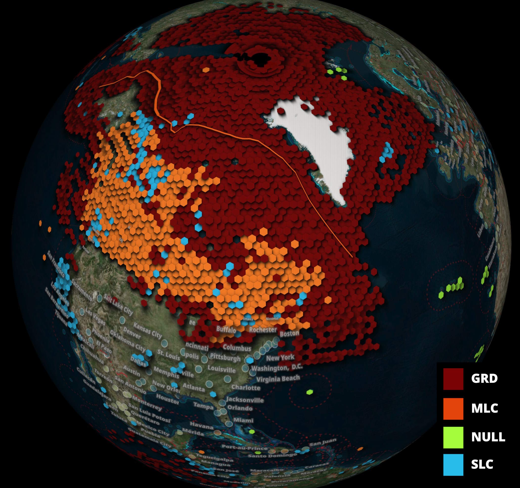
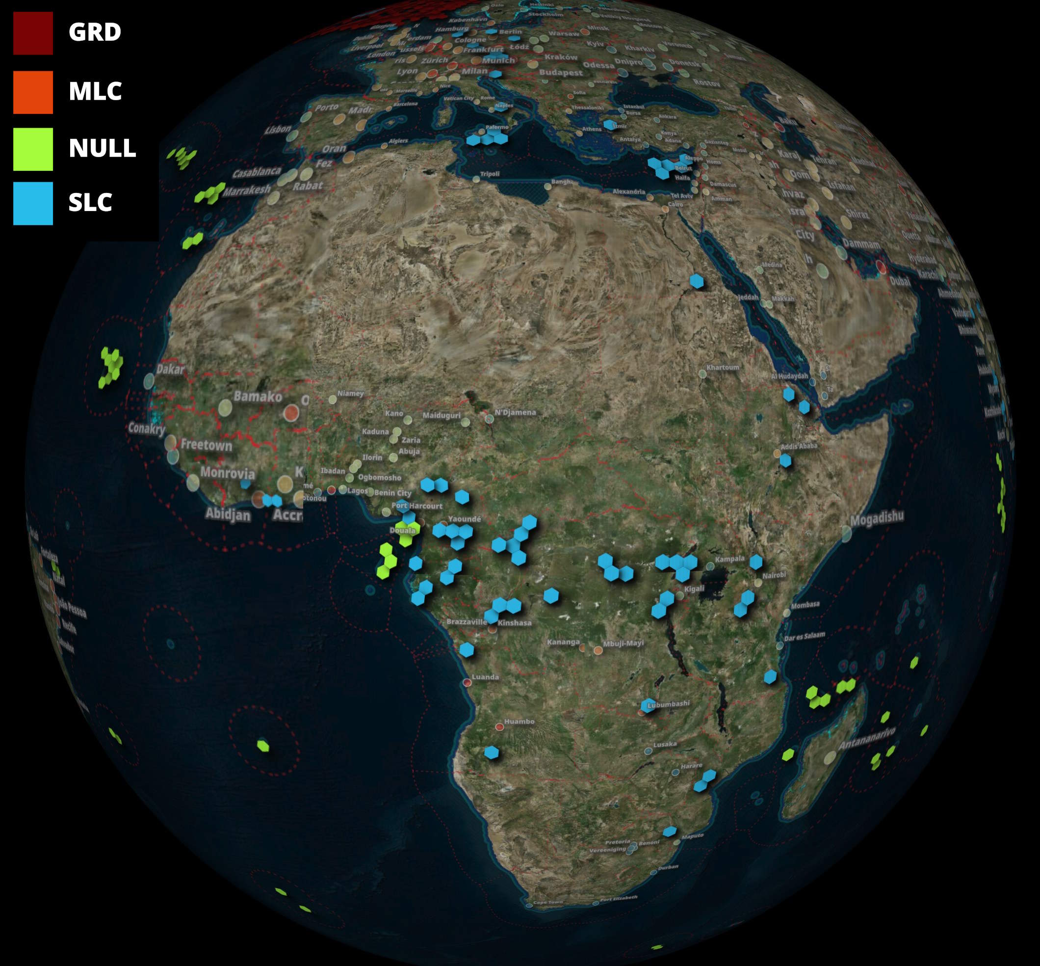
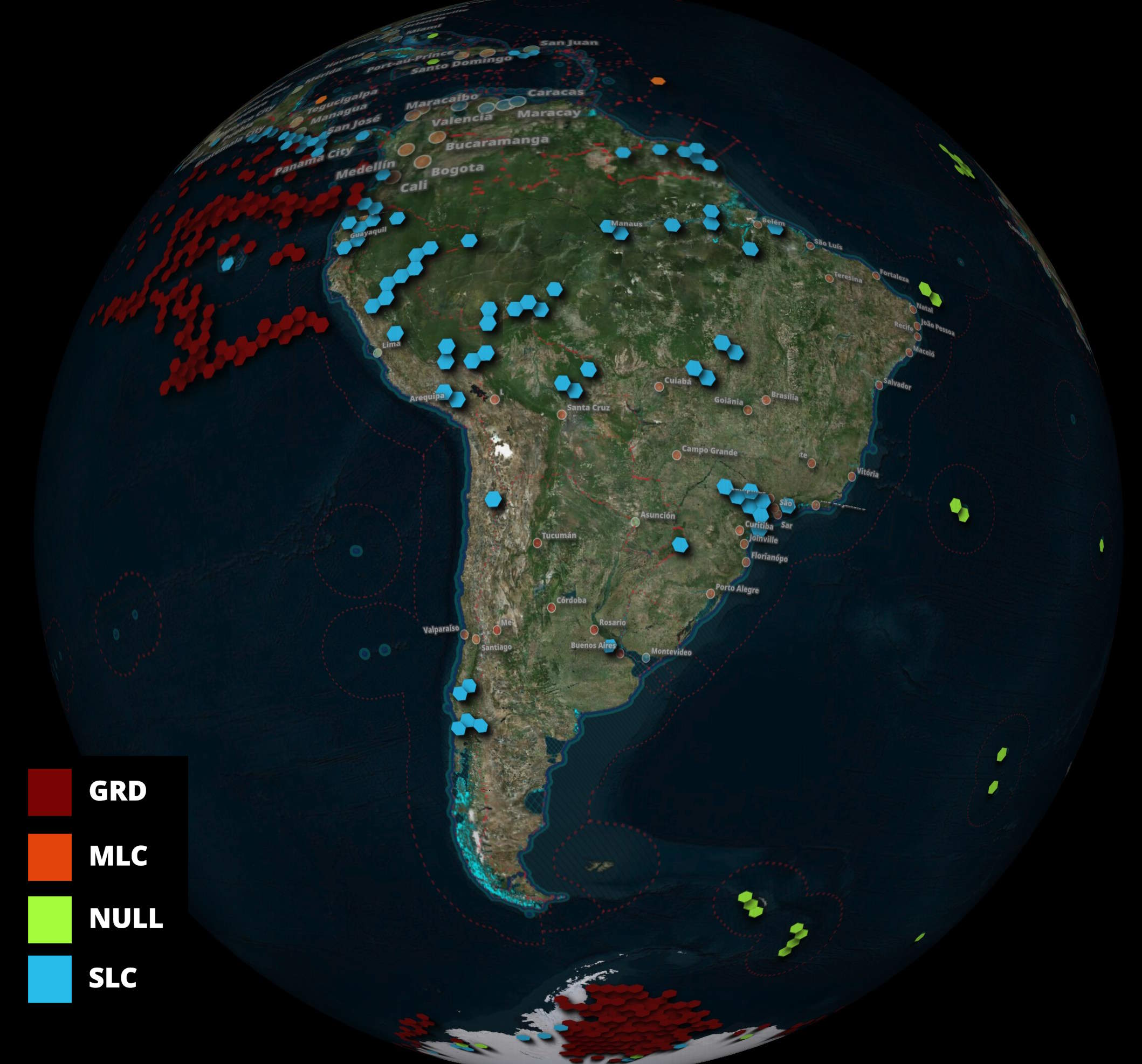
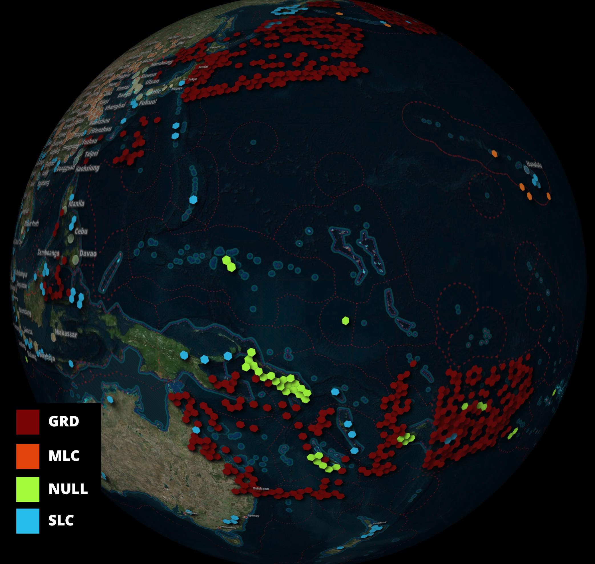
Gaps on the Map
The constellation is meant to help research climate change, but almost nowhere else in Antarctica, outside of where the newly-discovered Island is located, has had any images captured. I don't know if there is some sort of hardware limitation or if this area isn't a priority.
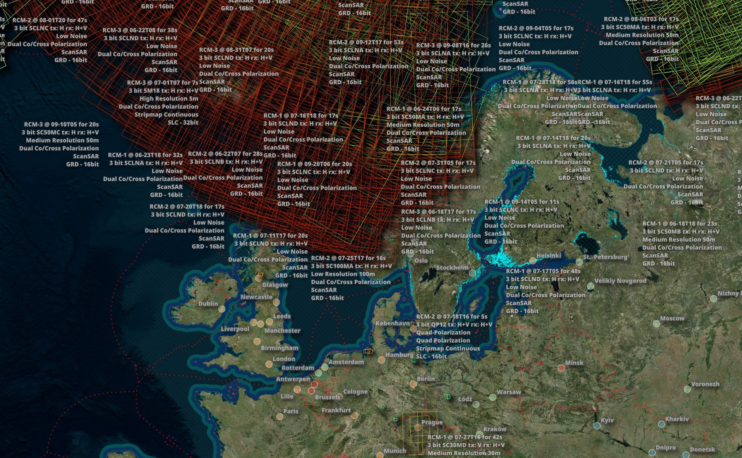
Very few European footprints land anywhere south of Norway. There are a handful of footprints over Prague, but not much else.
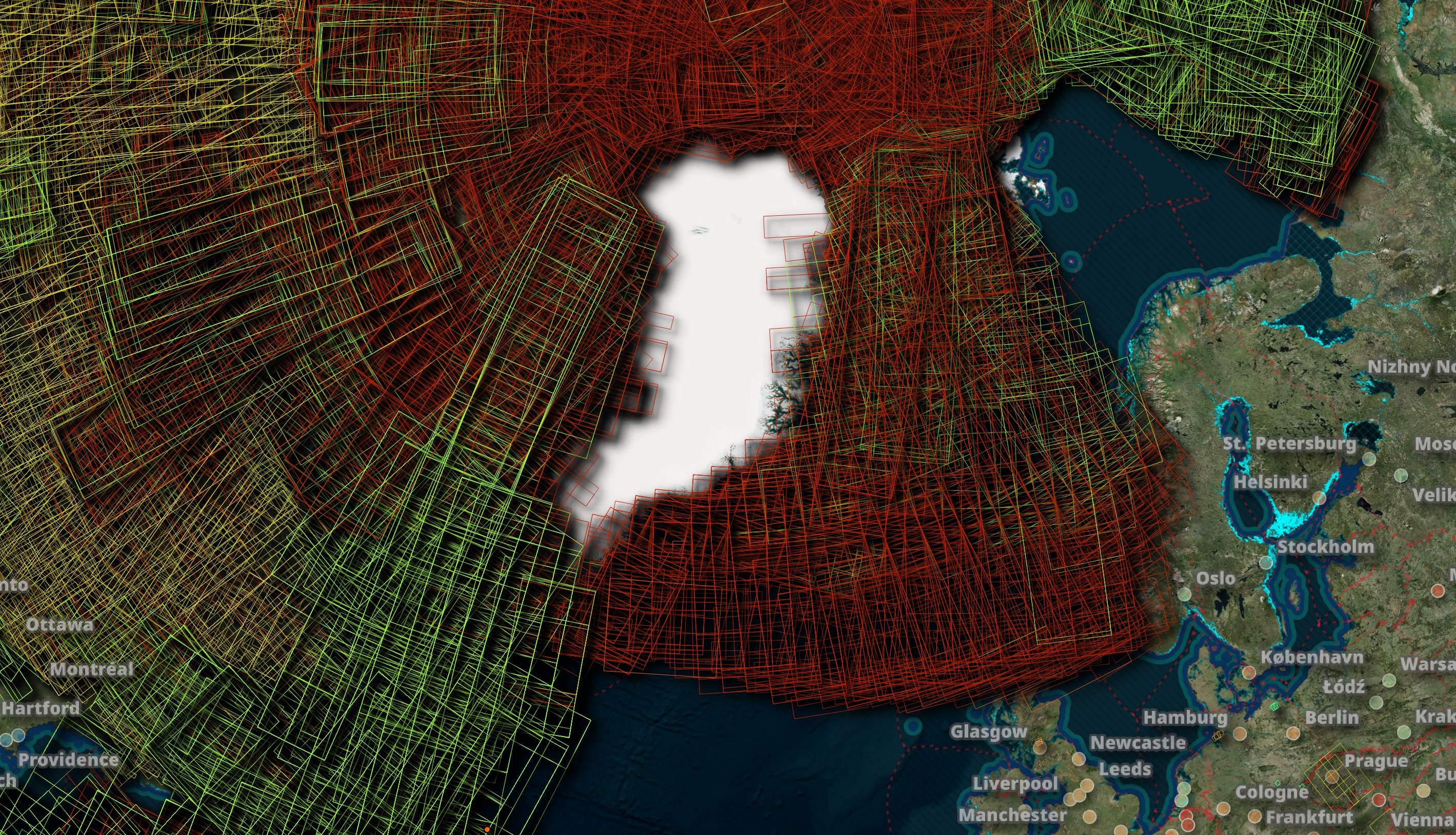
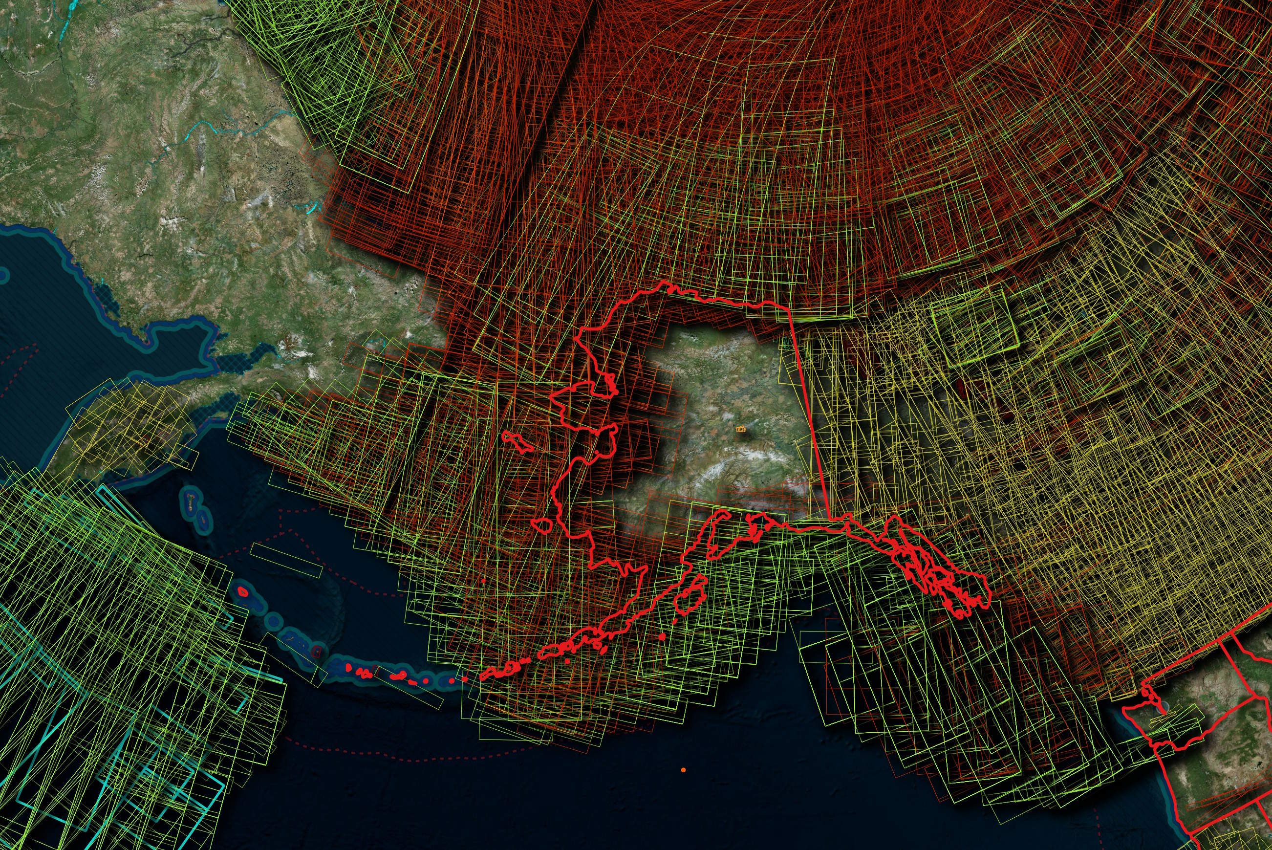
Landmasses in general are often overlooked compared to their coastlines. These are the footprints around Greenland and Alaska.
I can't imagine how they're not imaging anything in the Middle East or any other conflict-prone part of the world. But with that said, I can't find any patterns which suggest censorship in this list of footprints.
The Canadian Space Agency (CSA) has other assets which GCAT reports as being in orbit. It could just be that RCM's responsibilities are very narrow.
$ ~/duckdb
SELECT   Name,
         JCAT,
         Manufacturer,
         Owner,
         LDate,
         Launch_Tag,
         Bus,
         Shape,
         DryMass,
         Length,
         Diameter,
         Span,
         TotMass,
         OpOrbit,
         Apogee,
         Inc,
         Perigee,
         Status
FROM     'gcat/satcat.parquet'
WHERE    Owner = 'CSA'
ORDER BY Launch_Tag,
         Name;
┌────────────┬─────────┬──────────────┬─────────┬─────────────┬────────────┬──────────────┬────────────────────┬─────────┬────────┬──────────┬───────┬─────────┬─────────┬────────┬───────┬─────────┬──────────┐
│    Name    │  JCAT   │ Manufacturer │  Owner  │    LDate    │ Launch_Tag │     Bus      │       Shape        │ DryMass │ Length │ Diameter │ Span  │ TotMass │ OpOrbit │ Apogee │  Inc  │ Perigee │  Status  │
│  varchar   │ varchar │   varchar    │ varchar │   varchar   │  varchar   │   varchar    │      varchar       │ varchar │ float  │  float   │ float │  float  │ varchar │ int32  │ float │ varchar │ varchar  │
├────────────┼─────────┼──────────────┼─────────┼─────────────┼────────────┼──────────────┼────────────────────┼─────────┼────────┼──────────┼───────┼─────────┼─────────┼────────┼───────┼─────────┼──────────┤
│ CTA        │ S22214  │ CSA          │ CSA     │ 1992 Oct 22 │ 1992-070   │ CTA          │ Pan                │ 82      │    2.1 │      0.5 │   2.1 │    82.0 │ LLEO/I  │    215 │ 28.46 │ 207     │ Attached │
│ Radarsat   │ S23710  │ SPARM/BALL   │ CSA     │ 1995 Nov  4 │ 1995-059   │ RME/BCP-2000 │ Box + 2 Pan        │ 2750    │    4.2 │      2.8 │  15.0 │  2750.0 │ LEO/S   │    792 │ 98.58 │ 789     │ In orbit │
│ MOST       │ S27843  │ DYN          │ CSA     │ 2003 Jun 30 │ 2003-031   │ MOST         │ Box                │ 60      │    0.3 │      0.7 │   0.7 │    60.0 │ LEO/S   │    832 │ 98.72 │ 818     │ Renamed  │
│ SCISAT-1   │ S27858  │ BRIS         │ CSA     │ 2003 Aug 13 │ 2003-036   │ MAC-100      │ Cyl                │ 150     │    0.6 │      1.1 │   1.1 │   150.0 │ LEO/I   │    654 │ 73.94 │ 641     │ In orbit │
│ Radarsat-2 │ S32382  │ THALA        │ CSA     │ 2007 Dec 14 │ 2007-061   │ Prima        │ Box + 2 Pan        │ 2200    │    3.2 │      1.3 │  15.0 │  2300.0 │ LEO/S   │    798 │ 98.62 │ 791     │ In orbit │
│ NEOSSat    │ S39089  │ MSCI         │ CSA     │ 2013 Feb 25 │ 2013-009   │ MOST?        │ Box + 1 pan        │ 74      │    1.8 │      0.4 │   1.8 │    74.0 │ LEO/S   │    786 │ 98.63 │ 771     │ In orbit │
│ CASSIOPE   │ S39265  │ BALM/MDAM    │ CSA     │ 2013 Sep 29 │ 2013-055   │ MAC-200      │ Hex prism+antennae │ 481     │    1.4 │      1.8 │   2.0 │   481.0 │ LEO/I   │   1486 │  81.0 │ 325     │ In orbit │
│ RCM 1      │ S44322  │ BALM/MAXAR   │ CSA     │ 2019 Jun 12 │ 2019-033   │ MAC-200      │ Box+2 panels       │ 1400    │    5.0 │      1.4 │   7.0 │  1450.0 │ LLEO/S  │    604 │ 97.77 │ 584     │ In orbit │
│ RCM 2      │ S44323  │ BALM/MAXAR   │ CSA     │ 2019 Jun 12 │ 2019-033   │ MAC-200      │ Box+2 panels       │ 1400    │    5.0 │      1.4 │   7.0 │  1450.0 │ LLEO/S  │    603 │ 97.77 │ 584     │ In orbit │
│ RCM 3      │ S44324  │ BALM/MAXAR   │ CSA     │ 2019 Jun 12 │ 2019-033   │ MAC-200      │ Box+2 panels       │ 1400    │    5.0 │      1.4 │   7.0 │  1450.0 │ LLEO/S  │    603 │ 97.77 │ 584     │ In orbit │
└────────────┴─────────┴──────────────┴─────────┴─────────────┴────────────┴──────────────┴────────────────────┴─────────┴────────┴──────────┴───────┴─────────┴─────────┴────────┴───────┴─────────┴──────────┘
Expansion & Modern, Timely Feeds
It would be good to see the unversioned ZIP file these footprints are delivered in turned into a Parquet file. At a rate of 50,242 footprints over 98 days means ten years of footprints could be stored in a single file and not even break the 2M-record mark.
Also, an open imagery feed with timely publishing would be a huge step forward. Several commercial satellite operators are already doing this, including Wyvern, which is based in Edmonton and subject to all the same Global Affairs Canada regulations as RADARSAT is. I've lost count of how many academic papers I've seen with Sentinel imagery filling the pages.
An AIS feed could also provide a trusted, 3rd-party source and would do a lot to make shipping more transparent.
Lastly, given how RCM covers 95% of the planet's surface on any given day, what are the barriers to capturing and delivering imagery of that 95% every day?