The US Federal Aviation Administration (FAA) maintains a system called the National Airspace System Resource (NASR). It produces feeds that are freely available and have been used by firms such as Jeppesen for producing aviation charts.
Jesse McGraw has been working on two GitHub repositories for the past 12 years that convert these feeds into SQLite3 databases that can then be rendered in QGIS.
His first repository contains a QGIS workspace as well as a BASH script that downloads SVGs, CSVs, Natural Earth Shapefiles from a Dropbox link.
His second repository contains an ETL codebase and is made up of 4,039 lines of Python. Its earliest commit was in 2014 and has received updates as recently as three weeks ago. This codebase can be run on a regular basis and in order to the aviation charts up to date with the latest FAA data.
In this post, I'll analyse the map produced and its underlying datasets.
My Workstation
I'm using a 5.7 GHz AMD Ryzen 9 9950X CPU. It has 16 cores and 32 threads and 1.2 MB of L1, 16 MB of L2 and 64 MB of L3 cache. It has a liquid cooler attached and is housed in a spacious, full-sized Cooler Master HAF 700 computer case.
The system has 96 GB of DDR5 RAM clocked at 4,800 MT/s and a 5th-generation, Crucial T700 4 TB NVMe M.2 SSD which can read at speeds up to 12,400 MB/s. There is a heatsink on the SSD to help keep its temperature down. This is my system's C drive.
The system is powered by a 1,200-watt, fully modular Corsair Power Supply and is sat on an ASRock X870E Nova 90 Motherboard.
I'm running Ubuntu 24 LTS via Microsoft's Ubuntu for Windows on Windows 11 Pro. In case you're wondering why I don't run a Linux-based desktop as my primary work environment, I'm still using an Nvidia GTX 1080 GPU which has better driver support on Windows and ArcGIS Pro only supports Windows natively.
Installing Prerequisites
I'll use Python, jq and SQLite3 to help analyse the data in this post.
$ sudo add-apt-repository ppa:deadsnakes/ppa
$ sudo apt update
$ sudo apt install \
    jq \
    libsqlite3-mod-spatialite \
    python3-pip \
    python3.12-venv
I'll set up a Python Virtual Environment and install the FAA NASR ETL codebase.
$ python3 -m venv ~/.aviation_maps
$ source ~/.aviation_maps/bin/activate

$ git clone \
    https://github.com/jlmcgraw/processFaaData \
    ~/processFaaData
$ cd ~/processFaaData
$ pip install .
I'll use DuckDB, along with its H3, JSON, Lindel, Parquet and Spatial extensions in this post.
$ cd ~
$ wget -c https://github.com/duckdb/duckdb/releases/download/v1.5.1/duckdb_cli-linux-amd64.zip
$ unzip -j duckdb_cli-linux-amd64.zip
$ chmod +x duckdb
$ ~/duckdb
INSTALL h3 FROM community;
INSTALL lindel FROM community;
INSTALL json;
INSTALL parquet;
INSTALL spatial;
I'll set up DuckDB to load every installed extension each time it launches.
$ vi ~/.duckdbrc
.timer on
.width 180
LOAD h3;
LOAD lindel;
LOAD json;
LOAD parquet;
LOAD spatial;
The maps in this post were rendered with QGIS version 4.0.2. QGIS is a desktop application that runs on Windows, macOS and Linux. The application has grown in popularity in recent years and has ~15M application launches from users all around the world each month.
The maps in this post use the Droid Sans and Liberation Sans fonts.
An Aviation Chart Template
I'll clone the repository containing the QGIS workspace template (Aviation map.qgs) along with the script to pull down some of its assets.
$ git clone \
    https://github.com/jlmcgraw/aviationMap \
    ~/aviationMap
$ cd ~/aviationMap
The following will download a tar file from Dropbox. This codebase is more than a decade old and I suspect that if built from scratch today, these assets would just sit in the repository as is.
$ bash -x freshenLocalData.sh
Chart Assets
Below, I'll break down the contents by file type in the data.tar.xz file pulled off of Dropbox.
$ tar -tvf data.tar.xz > contents.txt
$ ~/duckdb
CREATE OR REPLACE TABLE contents AS
    SELECT file_size: SPLIT(TRIM(SPLIT(column0, 'jlmcgraw')[-1]), ' ')[1]::INT,
           file_path: SPLIT(column0, 'data/')[-1],
           file_type: IF(file_path LIKE '%.%',
                         LOWER(SPLIT(file_path, '.')[-1]),
                         NULL)
    FROM   READ_CSV('contents.txt', header=False);
Most of the content is SQLite3 files followed by Shapefiles. Most of the Shapefiles were sourced from Natural Earth.
SELECT   mb: CEIL(SUM(file_size) / 1024 ** 2)::INT,
         file_type
FROM     contents
GROUP BY 2
ORDER BY 1 DESC;
┌───────┬───────────┐
│  mb   │ file_type │
│ int32 │  varchar  │
├───────┼───────────┤
│   526 │ sqlite    │
│   166 │ shp       │
│   127 │ png       │
│    53 │ csv       │
│    43 │ dbf       │
│     7 │ tif       │
│     7 │ qix       │
│     5 │ ovr       │
│     3 │ shx       │
│     2 │ html      │
│     1 │ pdf       │
│     1 │ prj       │
│     1 │ txt       │
│     1 │ qpj       │
│     1 │ tsv       │
│     1 │ sh        │
│     1 │ xml       │
│     1 │ svg       │
│     1 │ md        │
│     1 │ NULL      │
└───────┴───────────┘
Four of the SQLite3 databases are placeholders. They do contain data but it is out of date. I suspect they're here just so there is something to see if you don't refresh the dataset, which I'll do later on in this post.
SELECT   file_size,
         file_path
FROM     contents
WHERE    file_type = 'sqlite'
ORDER BY file_size DESC;
┌───────────┬──────────────────────────────────────────────────┐
│ file_size │                    file_path                     │
│   int32   │                     varchar                      │
├───────────┼──────────────────────────────────────────────────┤
│ 238960640 │ databases/spatialite_nasr.sqlite                 │
│ 171323392 │ databases/edai.sqlite                            │
│  49068032 │ databases/ourAirports.sqlite                     │
│  41348096 │ databases/mef_spatialite.sqlite                  │
│  25546752 │ databases/special_use_airspace_spatialite.sqlite │
│  24641536 │ databases/controlled_airspace_spatialite.sqlite  │
└───────────┴──────────────────────────────────────────────────┘
These are the raster assets listed from largest to smallest.
SELECT   file_size,
         file_path
FROM     contents
WHERE    file_type IN ('png', 'tif')
ORDER BY file_size DESC;
┌───────────┬────────────────────────────────────────┐
│ file_size │ file_path │
│ int32 │ varchar │
├───────────┼────────────────────────────────────────┤
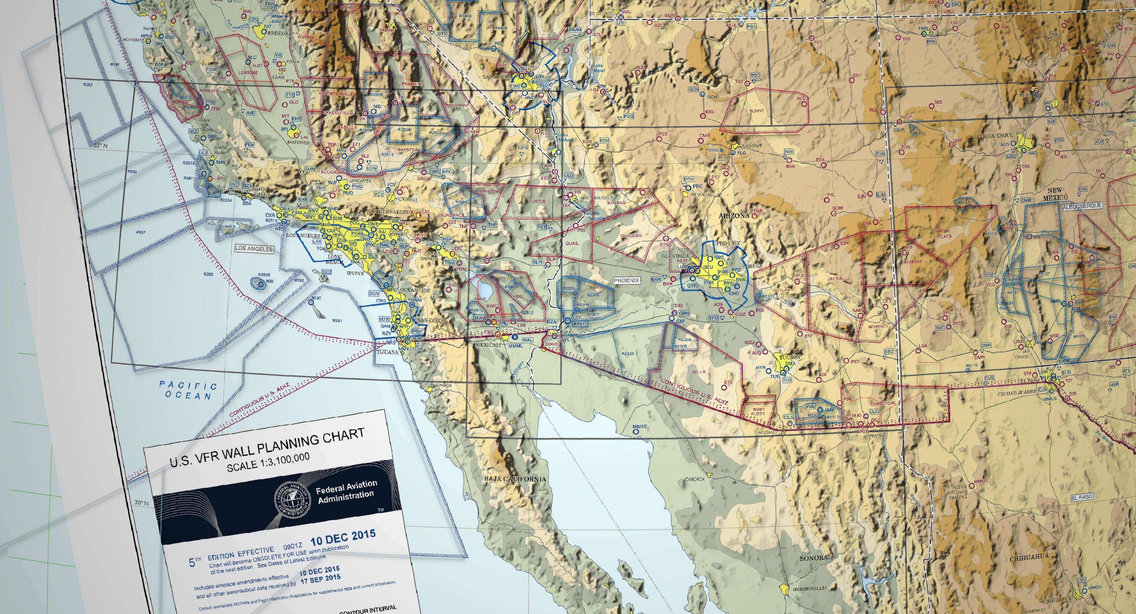
│ 83762662 │ U_S_VFR_Wall_Planning_Chart-warped.png │
│ 27300037 │ US_IFR_PLAN_EAST-warped.png │
│ 21132143 │ US_IFR_PLAN_WEST-warped.png │
│ 459799 │ sample_plates/00375IL28L.tif │
│ 436578 │ sample_plates/00375IL19L.tif │
│ 436069 │ sample_plates/00375IL28R.tif │
│ 417959 │ sample_plates/00375IPRM28L.tif │
│ 412942 │ sample_plates/00375LDAPRM28R.tif │
│ 409372 │ sample_plates/00375I28LSAC2.tif │
│ 390600 │ sample_plates/00375I28RSAC1.tif │
│ 390360 │ sample_plates/00375I28RC2_3.tif │
│ 387791 │ sample_plates/00375LDAD28R.tif │
│ 368050 │ sample_plates/00375RPRMX28R.tif │
│ 364701 │ sample_plates/00375RPRM28L.tif │
│ 362249 │ sample_plates/00375R28L.tif │
│ 338269 │ sample_plates/00375RX28R.tif │
│ 332126 │ sample_plates/00375RZ28R.tif │
│ 327189 │ sample_plates/00375R19L.tif │
│ 309869 │ sample_plates/00375R19R.tif │
│ 306458 │ sample_plates/00375RRY28R.tif │
│ 300011 │ sample_plates/00375RRZ10R.tif │
│ 282548 │ sample_plates/00375R10L.tif │
│ 280525 │ sample_plates/00375RY10R.tif │
└───────────┴────────────────────────────────────────┘
These are the CSV files.
SELECT   file_size,
         file_path
FROM     contents
WHERE    file_type IN ('csv', 'tsv')
ORDER BY file_size DESC;
┌───────────┬──────────────────────────────────────────┐
│ file_size │                file_path                 │
│   int32   │                 varchar                  │
├───────────┼──────────────────────────────────────────┤
│  18134248 │ iap-points.csv                           │
│   6402203 │ star-points.csv                          │
│   6077366 │ iap-lines.csv                            │
│   6040104 │ stars-points.csv                         │
│   5803819 │ weather/tafs.cache.csv                   │
│   5091964 │ sid-points.csv                           │
│   2004836 │ star-lines.csv                           │
│   1915010 │ stars-lines.csv                          │
│   1885205 │ sid-lines.csv                            │
│    876734 │ weather/metars.cache.csv                 │
│    209506 │ tfr/mergedTfrs.csv                       │
│    179412 │ weather/aircraftreports.cache.csv        │
│     93948 │ mora.csv                                 │
│     24679 │ weather/airsigmets.cache.csv             │
│     16378 │ artccGeometry.csv                        │
│       167 │ tile_layer_definitions/OpenStreetMap.tsv │
└───────────┴──────────────────────────────────────────┘
From the FAA to SQLite
I'll run a tool that will take the data the FAA currently has published and produce SQLite3 databases of their contents.
$ mkdir -p ~/FAA_NASR
$ cd ~/FAA_NASR

$ nasr fetch
$ nasr build
The above produced four SQLite3 files totalling 1.2 GB.
$ du -hsc *.sqlite
288M    class_airspace_spatialite.sqlite
572M    edai_spatialite.sqlite
317M    nasr.sqlite
12M     special_use_airspace_spatialite.sqlite
1.2G    total
I'll copy the above SQLite3 files into the map's databases folder.
$ cp *.sqlite ~/aviationMap/data/databases/
FAA Source Data Breakdown
The source data that built the SQLite3 files was a little under 2 GB.
$ python3
from pathlib import Path

with open('contents.json', 'w') as f:
    for path in Path('local_data').rglob('*'):
        f.write(json.dumps({'file_path': str(path),
                            'num_bytes': path.stat().st_size}) + '\n')
$ ~/duckdb
CREATE OR REPLACE TABLE contents AS
    SELECT *,
           feed: SPLIT(file_path, '/')[2],
           section: IF(SPLIT(file_path, '/')[3] NOT LIKE '%.%',
                       SPLIT(file_path, '/')[3],
                       NULL),
           file_type: IF(file_path LIKE '%.%' AND LENGTH(SPLIT(file_path, '.')[-1]) == 3,
                         LOWER(SPLIT(file_path, '.')[-1]),
                         NULL)
    FROM   READ_JSON('contents.json');


SELECT   mb: CEIL(SUM(num_bytes) / 1024 ** 2)::INT,
         feed
FROM     contents
WHERE    feed NOT ILIKE '%.zip'
GROUP BY 2
ORDER BY 1 DESC;
┌───────┬────────────────────────────────────────┐
│  mb   │                  feed                  │
│ int32 │                varchar                 │
├───────┼────────────────────────────────────────┤
│  1122 │ 28DaySubscription_Effective_2026-05-14 │
│   512 │ edai_extracted                         │
│   222 │ edai_downloads                         │
│    92 │ dof                                    │
└───────┴────────────────────────────────────────┘
Almost all of the TXT files are fixed-width CSVs. CSVs and TXTs together added up to ~678 MB uncompressed when I ran this.
There are 743 MB+ of Shapefiles that are uncompressed and the ZIP files within the EDAI feed are mostly packaging yet more Shapefiles.
WITH a AS (
    SELECT   num_bytes: CEIL(SUM(num_bytes) / 1024 ** 2)::INT,
             feed:      SPLIT(feed, '_Effective')[1],
             file_type
    FROM     contents
    WHERE    feed NOT ILIKE '%.zip'
    GROUP BY 2, 3
    ORDER BY 1 DESC
)
PIVOT    a
ON       feed
USING    SUM(num_bytes)
GROUP BY file_type
ORDER BY 2 DESC;
┌───────────┬───────────────────┬────────┬────────────────┬────────────────┐
│ file_type │ 28DaySubscription │  dof   │ edai_downloads │ edai_extracted │
│  varchar  │      int128       │ int128 │     int128     │     int128     │
├───────────┼───────────────────┼────────┼────────────────┼────────────────┤
│ txt       │               481 │   NULL │           NULL │           NULL │
│ shp       │               368 │   NULL │           NULL │            375 │
│ csv       │               105 │     92 │           NULL │           NULL │
│ zip       │                85 │   NULL │            222 │           NULL │
│ gfs       │                28 │   NULL │           NULL │           NULL │
│ dbf       │                25 │   NULL │           NULL │            131 │
│ xml       │                23 │   NULL │           NULL │              1 │
│ xsd       │                 5 │   NULL │           NULL │           NULL │
│ pdf       │                 4 │   NULL │           NULL │           NULL │
│ doc       │                 2 │   NULL │           NULL │           NULL │
│ shx       │                 1 │   NULL │           NULL │              6 │
│ NULL      │                 1 │      1 │              1 │              1 │
│ prj       │                 1 │   NULL │           NULL │              1 │
│ xls       │                 1 │   NULL │           NULL │           NULL │
│ cpg       │              NULL │   NULL │           NULL │              1 │
└───────────┴───────────────────┴────────┴────────────────┴────────────────┘
Aviation Charts in QGIS
I'll open the QGIS workspace file in the aviationMap folder and I'm greeted with the following map.
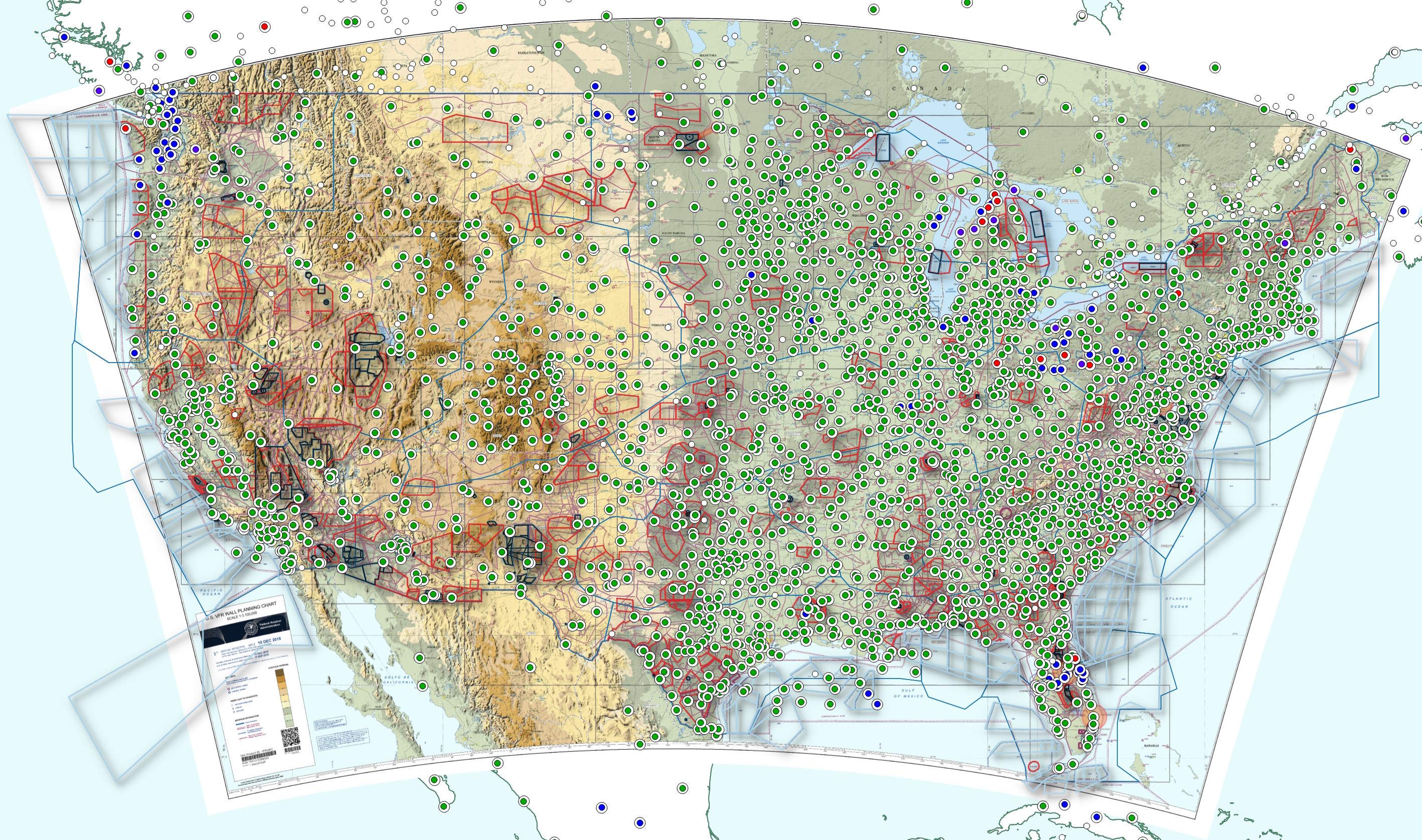
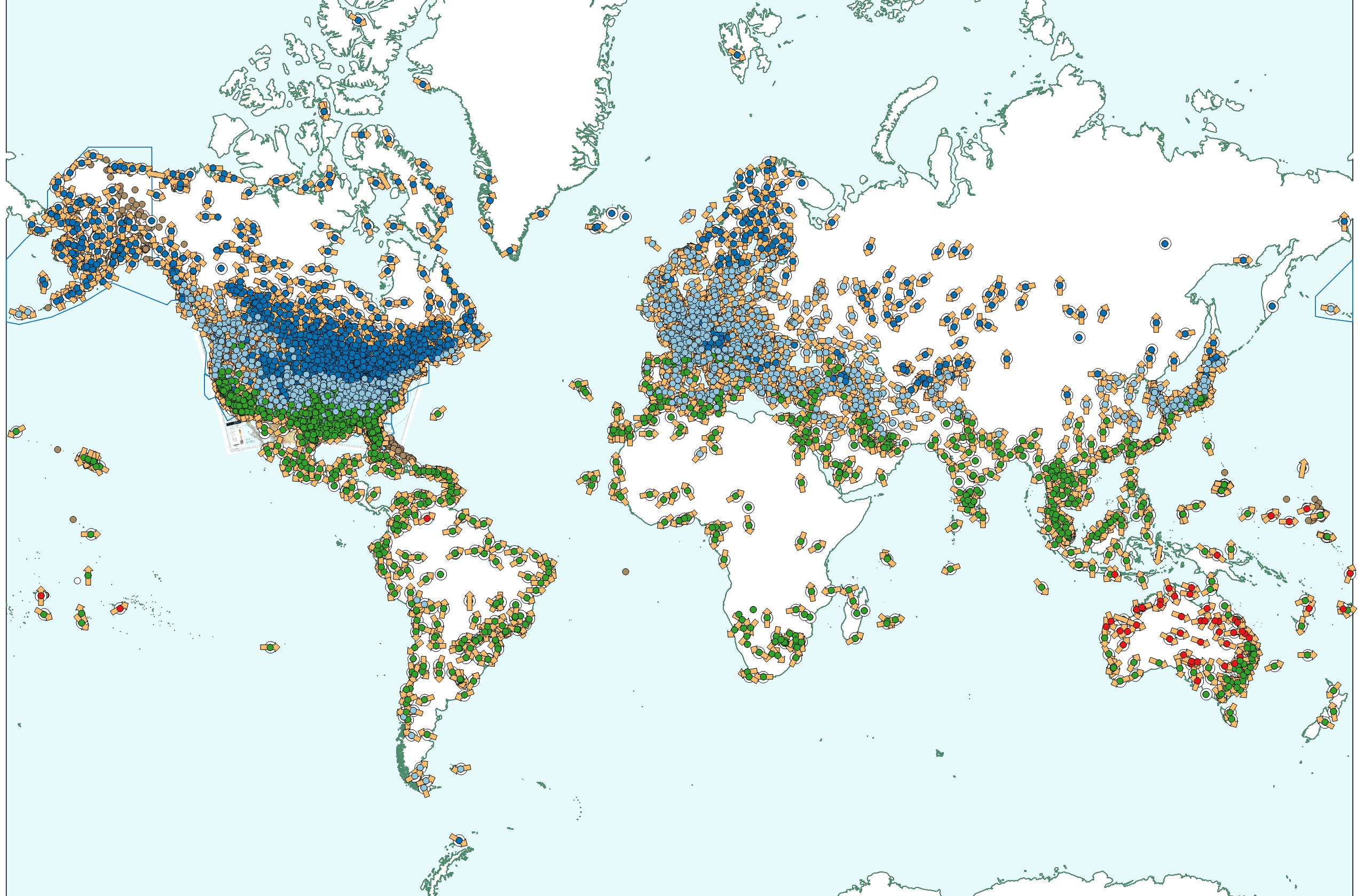
Not all data in this map covers areas outside of the US but there are some feeds that cover areas as remote as Antarctica.
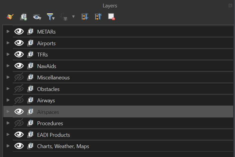
There are several groups that organise the contents of the map. Several of them will be hidden when you first open the map. Having every element visible at the same time will be visually overwhelming so toggling through each group is encouraged.
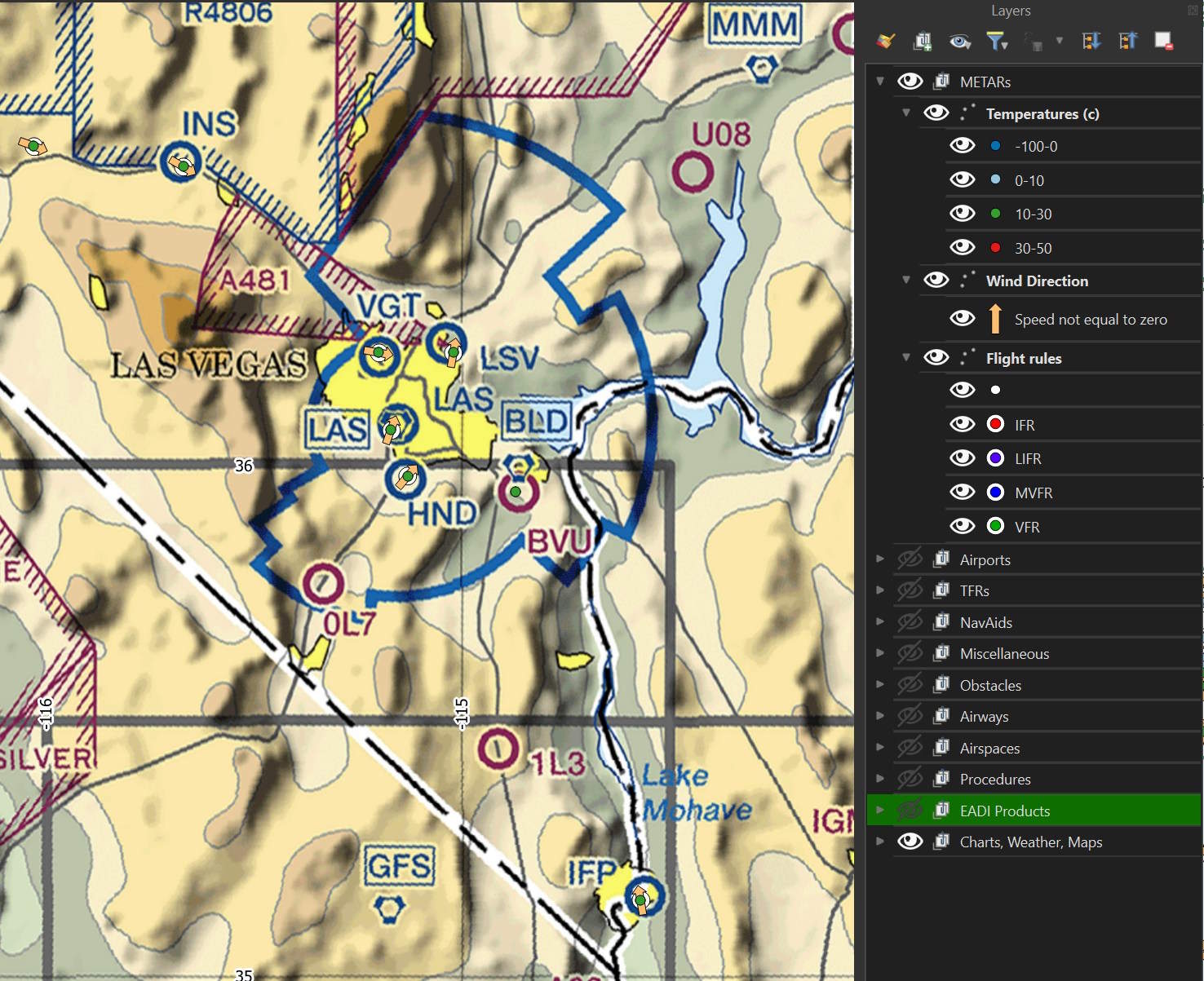
This is the METAR weather data in and around Las Vegas.
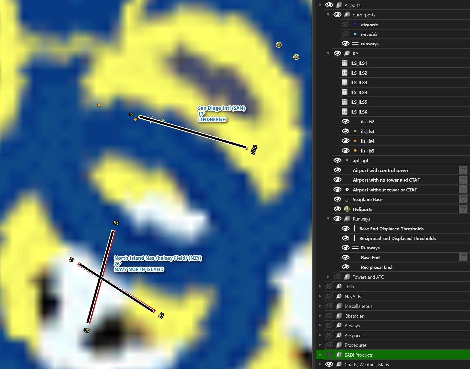
The basemap is a raster image so as you zoom into an airport, it can get pretty blurry. The following is the contents of the "Airports" layer with San Diego Intl. shown. The different classes of ILS are broken out and there is iconography differentiating airports with and without control towers.
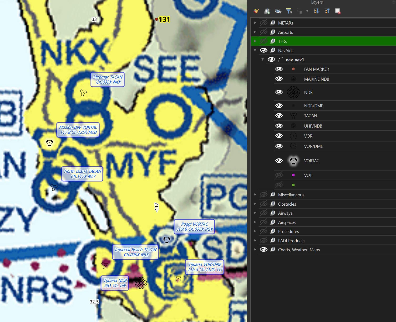
These are the different navigation aids layers.
Most of the miscellaneous group's contents will only appear when you're zoomed in pretty close to any one airport.
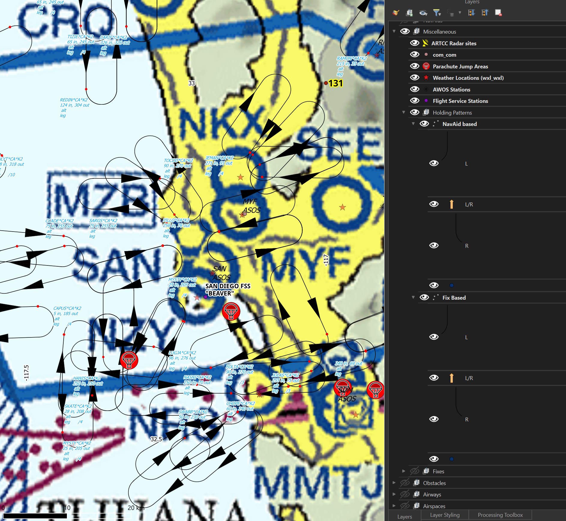
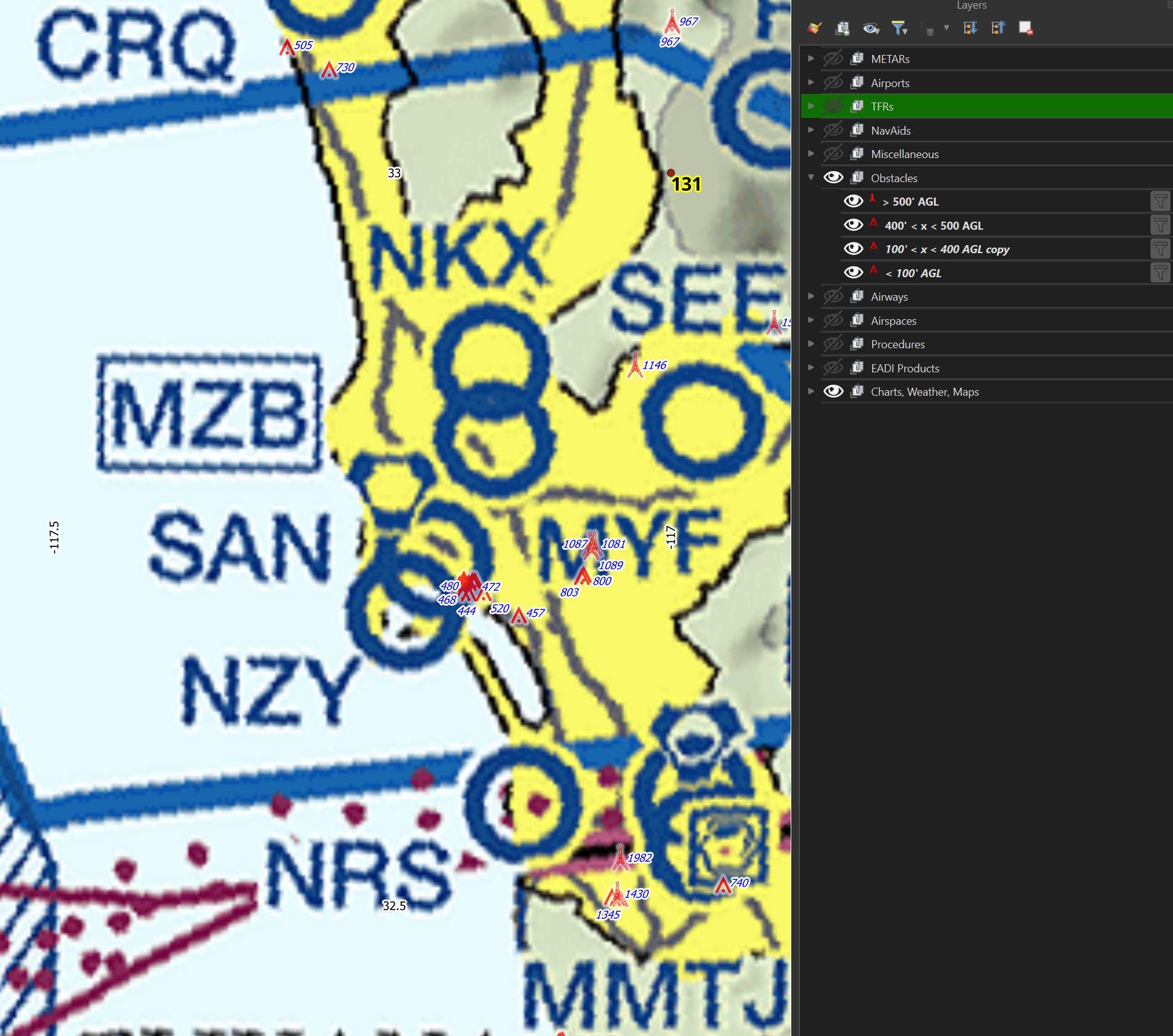
Obstacles will also only appear when zoomed in pretty far as well.
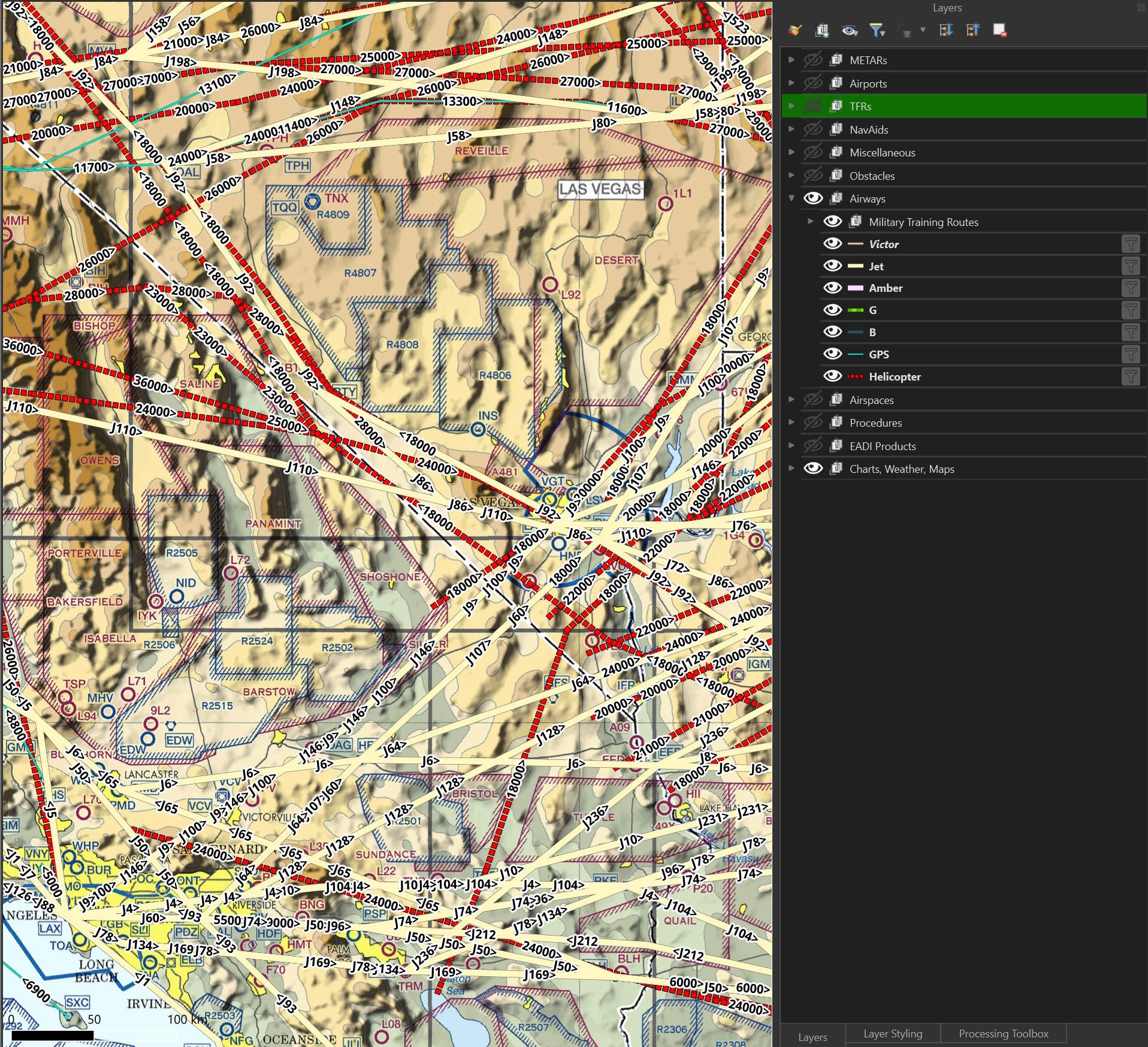
The contents of the Airways group will overwhelm the map pretty quickly. Toggling the individual routes of interest will make things much easier to digest.
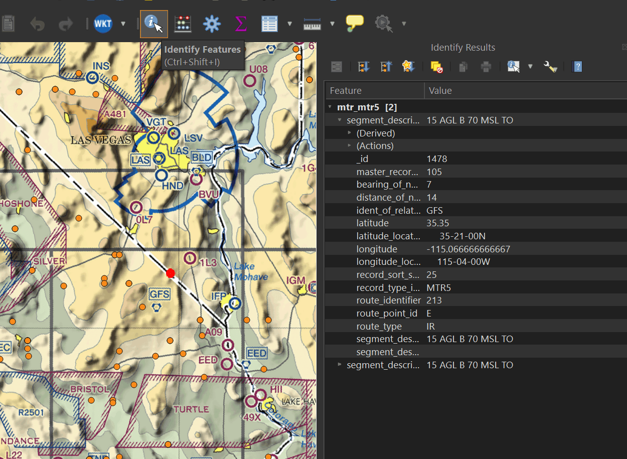
Every vector in the map will contain a varying amount of metadata. Clicking on any element with the "Identify Features" tool will bring up that item's properties.
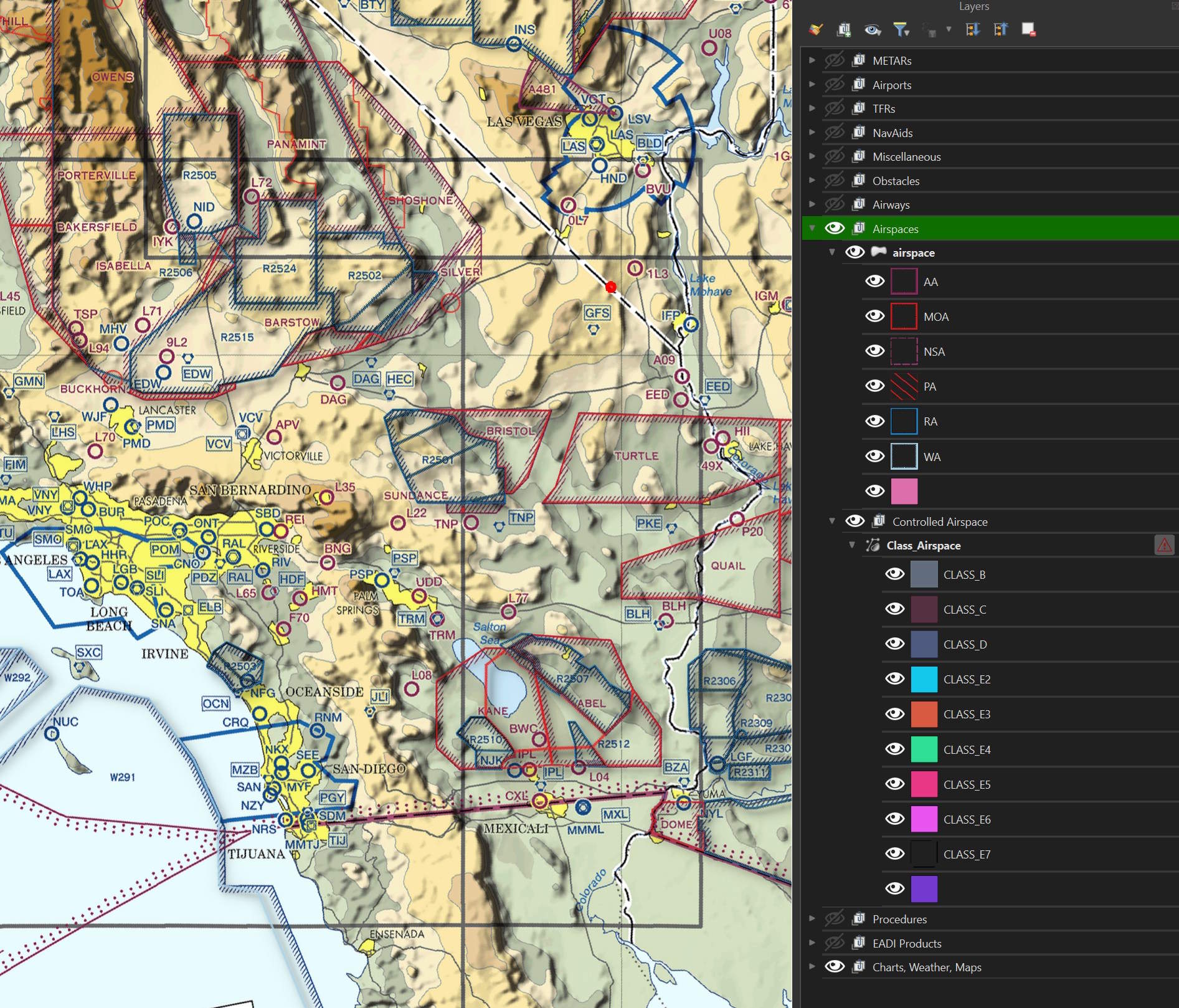
These are the Airspace classification layers. The controlled airspace data wouldn't load and I need to look into why this is.
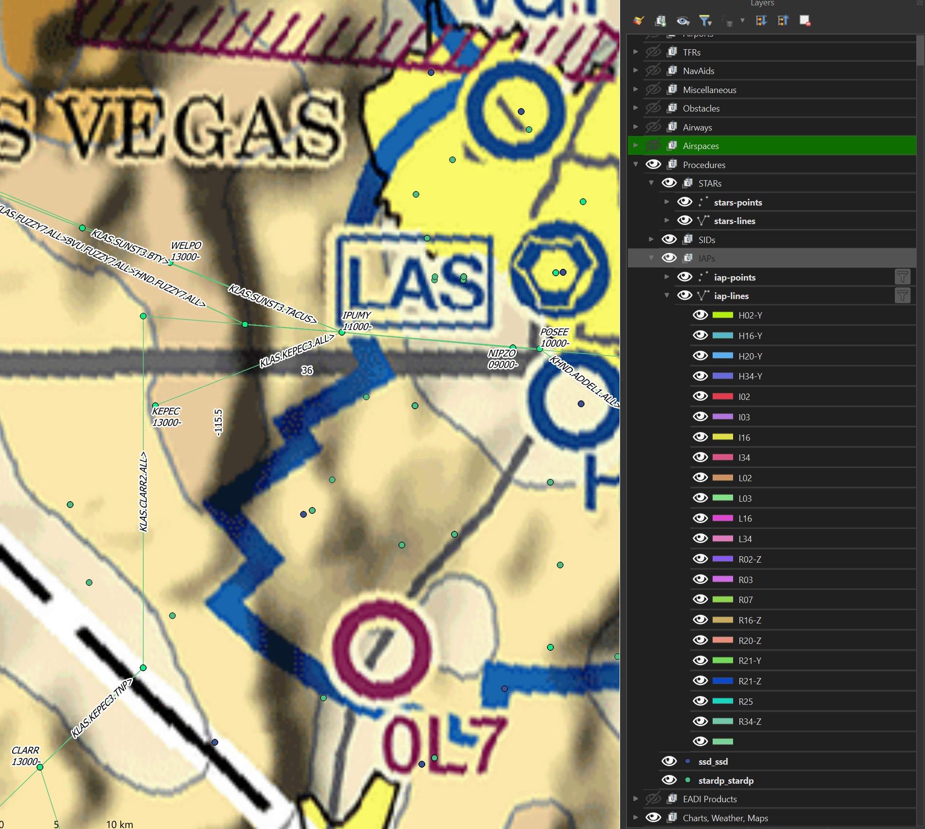
These are the procedures layers. You need to be zoomed in pretty close to any one airport for them to appear.
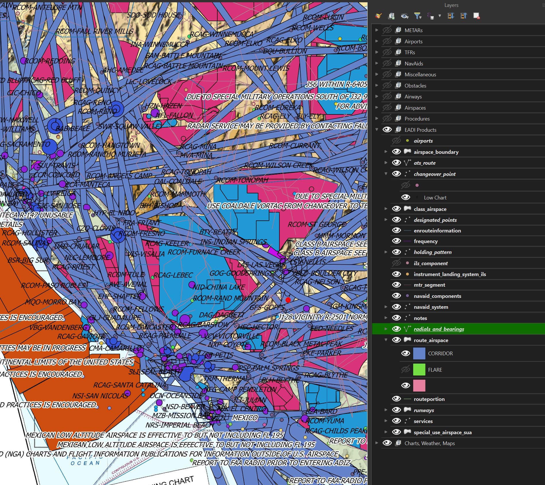
These are the EADI products layers.