The Global Airport Observations dataset is a Parquet-formatted, 1.75B-record collection of weather observations from 1940 up to today. The 655 MB Parquet file containing the 2024 data collected observation from thousands of stations in 14 countries. Often, stations reported observations hourly if not more frequently.
The data is hosted with one file per year on Cloudflare on behalf of the Source Cooperative. The data was originally sourced from the Iowa Environmental Mesonet.
In this post, I'll analyse this dataset.
My Workstation
I'm using a 5.7 GHz AMD Ryzen 9 9950X CPU. It has 16 cores and 32 threads and 1.2 MB of L1, 16 MB of L2 and 64 MB of L3 cache. It has a liquid cooler attached and is housed in a spacious, full-sized Cooler Master HAF 700 computer case.
The system has 96 GB of DDR5 RAM clocked at 4,800 MT/s and a 5th-generation, Crucial T700 4 TB NVMe M.2 SSD which can read at speeds up to 12,400 MB/s. There is a heatsink on the SSD to help keep its temperature down. This is my system's C drive.
The system is powered by a 1,200-watt, fully modular Corsair Power Supply and is sat on an ASRock X870E Nova 90 Motherboard.
I'm running Ubuntu 24 LTS via Microsoft's Ubuntu for Windows on Windows 11 Pro. In case you're wondering why I don't run a Linux-based desktop as my primary work environment, I'm still using an Nvidia GTX 1080 GPU which has better driver support on Windows and ArcGIS Pro only supports Windows natively.
Installing Prerequisites
I'll use jq to help analyse the data in this post.
$ sudo apt update
$ sudo apt install \
    jq
I'll use DuckDB, along with its H3, JSON, Lindel, Parquet and Spatial extensions in this post.
$ cd ~
$ wget -c https://github.com/duckdb/duckdb/releases/download/v1.5.1/duckdb_cli-linux-amd64.zip
$ unzip -j duckdb_cli-linux-amd64.zip
$ chmod +x duckdb
$ ~/duckdb
INSTALL h3 FROM community;
INSTALL lindel FROM community;
INSTALL json;
INSTALL parquet;
INSTALL spatial;
I'll set up DuckDB to load every installed extension each time it launches.
$ vi ~/.duckdbrc
.timer on
.width 180
LOAD h3;
LOAD lindel;
LOAD json;
LOAD parquet;
LOAD spatial;
The maps in this post were rendered with QGIS version 4.0.1. QGIS is a desktop application that runs on Windows, macOS and Linux. The application has grown in popularity in recent years and has ~15M application launches from users all around the world each month.
I used QGIS' HCMGIS plugin to add a satellite imagery basemaps from Bing and Esri to this post.
Friendly Field Names
I'll import the 2024 data into a DuckDB table. I'll structure the columns so that they explain themselves better than the original, abbreviated column names.
$ ~/duckdb asos.duckdb
CREATE OR REPLACE TABLE weather AS
    SELECT location: {
               altitude: alti,
               elevation: elevation,
               latitude: latitude,
               longitude: longitude,
               country: country,
               county: county,
               name: name,
               state: state,
               station: station,
               wfo: wfo,
           },
           time_: {
               tzname: tzname,
               valid: valid
           },
           temperature: {
               celsius: tmpc,
               fahrenheit: tmpf,
           },
           visibility: vsby,
           wind: {
               gust: gust,
               direction: drct,
               knots: sknt
           },
           dewpoint: {
               celsius: dwpc,
               fahrenheit: dwpf,
           },
           precipitation: {
               one_hour_inches: p01i,
               one_hour_metres: p01m
           },
           mean_sea_level_pressure: mslp,
           relative_humidity: relh
    FROM 'https://data.source.coop/dynamical/asos-parquet/year=2024/data.parquet';
This is the last observation made by Calgary International Airport in 2024.
$ echo "FROM     weather
        WHERE    location.name = 'CALGARY INTL'
        ORDER BY time_.valid DESC
        LIMIT    1" \
    | ~/duckdb -json asos.duckdb \
    | jq -S .
[
  {
    "dewpoint": {
      "celsius": -11.0,
      "fahrenheit": 12.2
    },
    "location": {
      "altitude": 30.15,
      "country": "CA",
      "county": null,
      "elevation": 1084.0,
      "latitude": 51.1139,
      "longitude": -114.0203,
      "name": "CALGARY INTL",
      "state": "CA_AB",
      "station": "CYYC",
      "wfo": null
    },
    "mean_sea_level_pressure": 1028.3,
    "precipitation": {
      "one_hour_inches": 0.0,
      "one_hour_metres": 0.0
    },
    "relative_humidity": 85.4,
    "temperature": {
      "celsius": -9.0,
      "fahrenheit": 15.8
    },
    "time_": {
      "tzname": "America/Edmonton",
      "valid": "2024-12-31 23:48:00+00"
    },
    "visibility": 1.5,
    "wind": {
      "direction": 60.0,
      "gust": null,
      "knots": 7.0
    }
  }
]
Below is a breakdown of unique values and NULL coverage across each column.
$ ~/duckdb asos.duckdb
SELECT   column_name,
         column_type,
         null_percentage,
         approx_unique,
         min,
         max
FROM     (SUMMARIZE
          SELECT * EXCLUDE(dewpoint,
                           location,
                           precipitation,
                           temperature,
                           time_,
                           wind),
                 dewpoint_celsius: dewpoint.celsius,
                 dewpoint_fahrenheit: dewpoint.fahrenheit,
                 location.*,
                 precipitation.*,
                 temperature_celsius: temperature.celsius,
                 temperature_fahrenheit: temperature.fahrenheit,
                 time_.*,
                 wind.*
          FROM weather);
┌─────────────────────────┬──────────────────────────┬─────────────────┬───────────────┬────────────────────────┬────────────────────────┐
│       column_name       │       column_type        │ null_percentage │ approx_unique │          min           │          max           │
│         varchar         │         varchar          │  decimal(9,2)   │     int64     │        varchar         │        varchar         │
├─────────────────────────┼──────────────────────────┼─────────────────┼───────────────┼────────────────────────┼────────────────────────┤
│ visibility              │ DOUBLE                   │            4.86 │           231 │ 0.0                    │ 1010009.0              │
│ mean_sea_level_pressure │ DOUBLE                   │           72.95 │          1947 │ 889.0                  │ 1131.3                 │
│ relative_humidity       │ DOUBLE                   │            0.55 │          7241 │ 0.52                   │ 100.42                 │
│ dewpoint_celsius        │ DOUBLE                   │            0.46 │           794 │ -98.0                  │ 37.11                  │
│ dewpoint_fahrenheit     │ DOUBLE                   │            0.46 │           806 │ -144.4                 │ 98.8                   │
│ altitude                │ DOUBLE                   │            4.16 │           866 │ 0.0                    │ 295.27                 │
│ elevation               │ DOUBLE                   │            0.00 │          2058 │ -499.14362             │ 3792.0                 │
│ latitude                │ DOUBLE                   │            0.00 │          3778 │ -45.0211               │ 82.5178                │
│ longitude               │ DOUBLE                   │            0.00 │          3485 │ -177.3756              │ 177.5667               │
│ country                 │ VARCHAR                  │            0.00 │            11 │ AU                     │ ZA                     │
│ county                  │ VARCHAR                  │           26.09 │          1294 │ Accomack               │ Zapata                 │
│ name                    │ VARCHAR                  │            0.00 │          4381 │ ABBOTSFORD             │ Zihuatanejo            │
│ state                   │ VARCHAR                  │            0.00 │            76 │ AK                     │ ZA                     │
│ station                 │ VARCHAR                  │            0.00 │          5698 │ 00U                    │ ZZV                    │
│ wfo                     │ VARCHAR                  │           26.09 │           126 │ ABQ                    │ VEF                    │
│ one_hour_inches         │ DOUBLE                   │            0.25 │           486 │ 0.0                    │ 75.69                  │
│ one_hour_metres         │ DOUBLE                   │            0.25 │           467 │ 0.0                    │ 1922.53                │
│ temperature_celsius     │ DOUBLE                   │            0.00 │           888 │ -66.89                 │ 242.0                  │
│ temperature_fahrenheit  │ DOUBLE                   │            0.00 │          1019 │ -88.4                  │ 467.6                  │
│ tzname                  │ VARCHAR                  │            0.00 │           111 │ Africa/Johannesburg    │ Pacific/Norfolk        │
│ valid                   │ TIMESTAMP WITH TIME ZONE │            0.00 │        592837 │ 2024-01-01 02:00:00+02 │ 2025-01-01 01:59:00+02 │
│ gust                    │ DOUBLE                   │           86.42 │           299 │ 0.0                    │ 402.0                  │
│ direction               │ DOUBLE                   │            4.54 │           229 │ 0.0                    │ 360.0                  │
│ knots                   │ DOUBLE                   │            1.30 │           562 │ 0.0                    │ 1796.11                │
└─────────────────────────┴──────────────────────────┴─────────────────┴───────────────┴────────────────────────┴────────────────────────┘
Canadian Data
The 2024 dataset has observations from 525 weather stations in Canada.
$ ~/duckdb asos.duckdb
SELECT   location.name,
         COUNT(*)
FROM     weather
WHERE    location.country = 'CA'
GROUP BY 1
ORDER BY 2 DESC;
┌──────────────────────┬──────────────┐
│         name         │ count_star() │
│       varchar        │    int64     │
├──────────────────────┼──────────────┤
│ ESQUIMALT HARBOUR    │        30370 │
│ INUKJUAK ARPT        │        25546 │
│ Dease Lake           │        24046 │
│ SCHEFFERVILLE A      │        22918 │
│ KUUJJUARAPIK ARPT    │        21664 │
│ PUVIRNITUQ           │        21509 │
│ BELLA BELLA CAMPBELL │        21413 │
│ MATAGAMI             │        21144 │
│ CHAPAIS              │        21119 │
│ PORT HAWKESBURY      │        20741 │
│ REVELSTOKE AIRPO     │        20329 │
│ GJOA HAVEN           │        20181 │
│ MUSKOKA              │        20044 │
│ Peawanuck            │        20001 │
│ SABLE ISLAND         │        19836 │
│ LA GRANDE IV ARP     │        19693 │
│ FORT SEVERN          │        19244 │
│ PETERBOROUGH         │        19207 │
│ WATERLOO             │        18946 │
│ PICKLE LAKE  A       │        18918 │
│    ·                 │           ·  │
│    ·                 │           ·  │
│    ·                 │           ·  │
│ UMIUJAQ              │         2413 │
│ PEORIA AGDM  ALTA    │         2407 │
│ OLDS AGDM  ALTA      │         2290 │
│ FORT RESOLUTION      │         2271 │
│ LOWER CARP LAKE  NWT │         2230 │
│ MORRIN AGDM  ALTA    │         2198 │
│ FOREMOST AGDM  ALTA  │         2196 │
│ FORT LIARD           │         2161 │
│ GRISE FIORD AIRPORT  │         2116 │
│ DE WEMINDJI          │         2074 │
│ ENCHANT AGDM  ALTA   │         2074 │
│ EASTMAIN RIVER       │         2066 │
│ BARNWELL AGDM  ALTA  │         2051 │
│ HOLMAN               │         1841 │
│ AKULIVIK             │         1793 │
│ OLD CROW             │         1767 │
│ FORT NORMAN AIRPORT  │         1688 │
│ ST. PAUL AGDM  ALTA  │         1572 │
│ SACHS HARBOUR        │         1526 │
│ WASKAGANISH AIRPORT  │         1144 │
└──────────────────────┴──────────────┘
Below, I'll produce a Parquet file with the locations of each station.
COPY (
    SELECT DISTINCT
           geometry: ST_ASWKB(ST_POINT(location.longitude,
                                       location.latitude)),
           location.name
    FROM   weather
    WHERE  location.country = 'CA'
) TO 'asos.canada.parquet' (
        FORMAT 'PARQUET',
        CODEC  'ZSTD',
        COMPRESSION_LEVEL 22,
        ROW_GROUP_SIZE 15000);
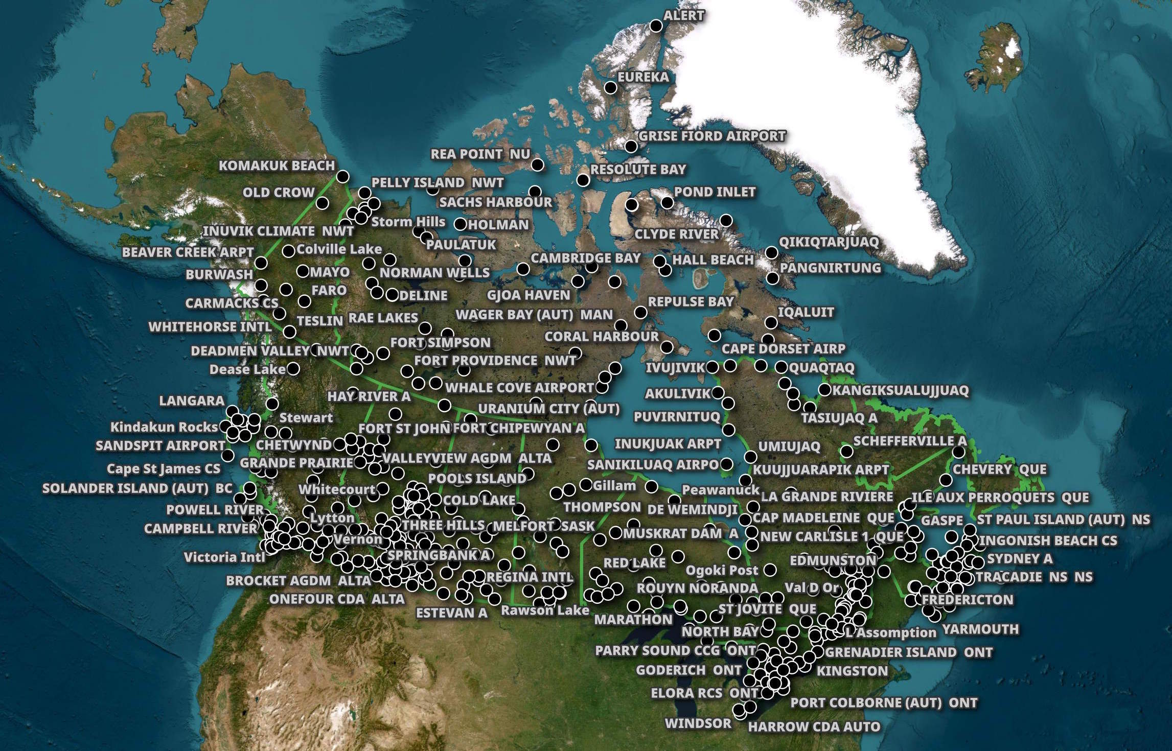
The whole of Canada looks well-covered.
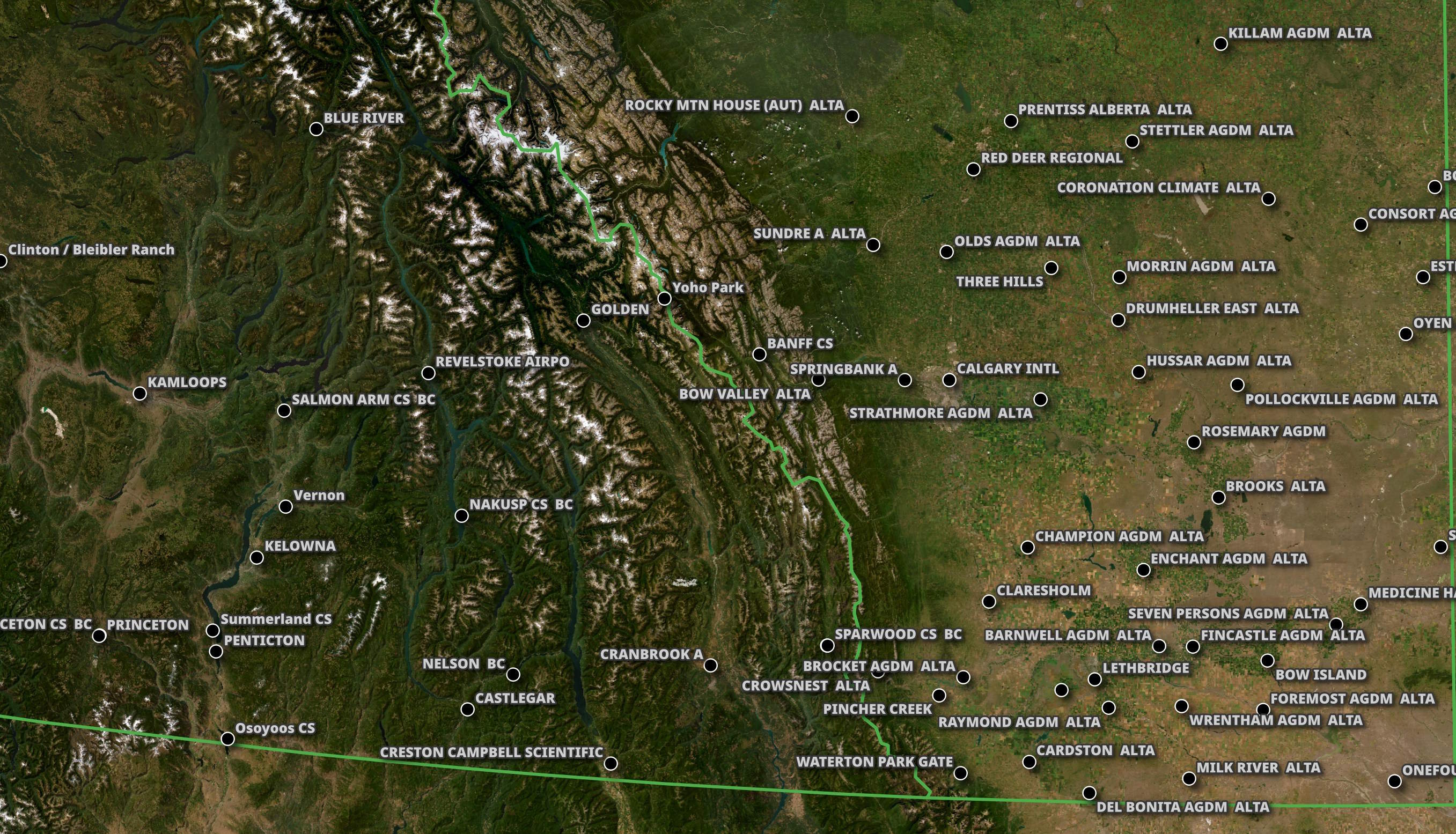
This shows the density of observation stations in Southern Alberta and BC.
Observation Frequency
Calgary Airport looks to submit at least one observation per hour, though several hours have even more.
$ ~/duckdb asos.duckdb
WITH a AS (
    SELECT   yyyy_ww: strftime(time_.valid, '%Y-%W'),
             day_num: strftime(time_.valid, '%u (%a)'),
             rec_num: COUNT(*)
    FROM     weather
    WHERE    location.name = 'CALGARY INTL'
    GROUP BY 1, 2
    ORDER BY 1, 2
)
PIVOT    a
ON       day_num
USING    SUM(rec_num)
GROUP BY yyyy_ww
ORDER BY yyyy_ww;
┌─────────┬─────────┬─────────┬─────────┬─────────┬─────────┬─────────┬─────────┐
│ yyyy_ww │ 1 (Mon) │ 2 (Tue) │ 3 (Wed) │ 4 (Thu) │ 5 (Fri) │ 6 (Sat) │ 7 (Sun) │
│ varchar │ int128  │ int128  │ int128  │ int128  │ int128  │ int128  │ int128  │
├─────────┼─────────┼─────────┼─────────┼─────────┼─────────┼─────────┼─────────┤
│ 2024-01 │      27 │      25 │      49 │      32 │      28 │      25 │      32 │
│ 2024-02 │      25 │      24 │      45 │      40 │      27 │      28 │      26 │
│ 2024-03 │      25 │      28 │      39 │      34 │      25 │      24 │      26 │
│ 2024-04 │      28 │      27 │      25 │      28 │      26 │      25 │      27 │
│ 2024-05 │      28 │      25 │      25 │      26 │      25 │      34 │      34 │
│ 2024-06 │      30 │      37 │      59 │      47 │      29 │      24 │      26 │
│ 2024-07 │      25 │      35 │      24 │      34 │      24 │      24 │      25 │
│ 2024-08 │      25 │      26 │      25 │      26 │      24 │      36 │      24 │
│ 2024-09 │      41 │      30 │      24 │      25 │      46 │      48 │      31 │
│ 2024-10 │      27 │      25 │      33 │      26 │      24 │      24 │      27 │
│ 2024-11 │      26 │      25 │      25 │      26 │      26 │      25 │      26 │
│ 2024-12 │      25 │      25 │      44 │      47 │      39 │      40 │      33 │
│ 2024-13 │      27 │      29 │      25 │      29 │      33 │      36 │      24 │
│ 2024-14 │      27 │      25 │      26 │      44 │      54 │      31 │      27 │
│ 2024-15 │      27 │      24 │      30 │      24 │      26 │      27 │      26 │
│ 2024-16 │      24 │      46 │      36 │      25 │      26 │      25 │      27 │
│ 2024-17 │      24 │      25 │      24 │      25 │      25 │      25 │      24 │
│ 2024-18 │      24 │      49 │      47 │      43 │      29 │      26 │      24 │
│ 2024-19 │      30 │      27 │      25 │      24 │      24 │      24 │      28 │
│ 2024-20 │      25 │      29 │      24 │      32 │      43 │      28 │      34 │
│    ·    │       · │       · │       · │       · │       · │       · │       · │
│    ·    │       · │       · │       · │       · │       · │       · │       · │
│    ·    │       · │       · │       · │       · │       · │       · │       · │
│ 2024-35 │      24 │      24 │      35 │      25 │      26 │      24 │      24 │
│ 2024-36 │      24 │      27 │      25 │      24 │      24 │      24 │      24 │
│ 2024-37 │      24 │      35 │      34 │      42 │      25 │      26 │      27 │
│ 2024-38 │      24 │      24 │      24 │      26 │      47 │      25 │      24 │
│ 2024-39 │      24 │      24 │      24 │      35 │      24 │      22 │      26 │
│ 2024-40 │      28 │      24 │      29 │      26 │      25 │      25 │      24 │
│ 2024-41 │      24 │      24 │      26 │      26 │      25 │      24 │      25 │
│ 2024-42 │      24 │      24 │      24 │      26 │      24 │      27 │      24 │
│ 2024-43 │      31 │      42 │      25 │      26 │      26 │      27 │      25 │
│ 2024-44 │      25 │      32 │      26 │      26 │      41 │      25 │      30 │
│ 2024-45 │      27 │      32 │      26 │      26 │      24 │      27 │      27 │
│ 2024-46 │      31 │      25 │      26 │      24 │      36 │      29 │      28 │
│ 2024-47 │      34 │      38 │      47 │      43 │      45 │      45 │      26 │
│ 2024-48 │      25 │      28 │      26 │      56 │      45 │      34 │      26 │
│ 2024-49 │      25 │      25 │      44 │      33 │      25 │      25 │      31 │
│ 2024-50 │      24 │      24 │      27 │      37 │      26 │      27 │      27 │
│ 2024-51 │      38 │      51 │      38 │      24 │      26 │      31 │      27 │
│ 2024-52 │      27 │      25 │      29 │      26 │      25 │      23 │      24 │
│ 2024-53 │      37 │      38 │    NULL │    NULL │    NULL │    NULL │    NULL │
│ 2025-00 │    NULL │    NULL │       5 │    NULL │    NULL │    NULL │    NULL │
└─────────┴─────────┴─────────┴─────────┴─────────┴─────────┴─────────┴─────────┘
Below is one such day with more than one observation per hour.
SELECT   time_.valid,
         temperature,
         visibility,
         wind
FROM     weather
WHERE    DATE(time_.valid) = '2024-01-11'::DATE
AND      location.name     = 'CALGARY INTL'
ORDER BY time_.valid;
┌──────────────────────────┬───────────────────────────────────────────┬────────────┬─────────────────────────────────────────────────────┐
│          valid           │                temperature                │ visibility │                        wind                         │
│ timestamp with time zone │ struct(celsius double, fahrenheit double) │   double   │ struct(gust double, direction double, knots double) │
├──────────────────────────┼───────────────────────────────────────────┼────────────┼─────────────────────────────────────────────────────┤
│ 2024-01-11 00:00:00+02   │ {'celsius': -21.0, 'fahrenheit': -5.8}    │        3.0 │ {'gust': 21.0, 'direction': 360.0, 'knots': 15.0}   │
│ 2024-01-11 00:54:00+02   │ {'celsius': -22.0, 'fahrenheit': -7.6}    │       2.25 │ {'gust': 18.0, 'direction': 20.0, 'knots': 13.0}    │
│ 2024-01-11 01:00:00+02   │ {'celsius': -22.0, 'fahrenheit': -7.6}    │        1.5 │ {'gust': 19.0, 'direction': 30.0, 'knots': 14.0}    │
│ 2024-01-11 02:00:00+02   │ {'celsius': -22.0, 'fahrenheit': -7.6}    │        2.5 │ {'gust': 17.0, 'direction': 30.0, 'knots': 12.0}    │
│ 2024-01-11 03:00:00+02   │ {'celsius': -23.0, 'fahrenheit': -9.4}    │        2.5 │ {'gust': 19.0, 'direction': 20.0, 'knots': 12.0}    │
│ 2024-01-11 03:47:00+02   │ {'celsius': -23.0, 'fahrenheit': -9.4}    │        8.0 │ {'gust': NULL, 'direction': 20.0, 'knots': 16.0}    │
│ 2024-01-11 04:00:00+02   │ {'celsius': -23.0, 'fahrenheit': -9.4}    │        8.0 │ {'gust': 22.0, 'direction': 20.0, 'knots': 15.0}    │
│ 2024-01-11 04:34:00+02   │ {'celsius': -23.0, 'fahrenheit': -9.4}    │        7.0 │ {'gust': 20.0, 'direction': 40.0, 'knots': 12.0}    │
│ 2024-01-11 05:00:00+02   │ {'celsius': -23.0, 'fahrenheit': -9.4}    │        7.0 │ {'gust': NULL, 'direction': 30.0, 'knots': 13.0}    │
│ 2024-01-11 06:00:00+02   │ {'celsius': -24.0, 'fahrenheit': -11.2}   │        7.0 │ {'gust': 19.0, 'direction': 30.0, 'knots': 12.0}    │
│ 2024-01-11 06:34:00+02   │ {'celsius': -24.0, 'fahrenheit': -11.2}   │        5.0 │ {'gust': 20.0, 'direction': 30.0, 'knots': 13.0}    │
│ 2024-01-11 07:00:00+02   │ {'celsius': -24.0, 'fahrenheit': -11.2}   │        4.0 │ {'gust': 17.0, 'direction': 40.0, 'knots': 12.0}    │
│ 2024-01-11 08:00:00+02   │ {'celsius': -24.0, 'fahrenheit': -11.2}   │        4.0 │ {'gust': NULL, 'direction': 50.0, 'knots': 15.0}    │
│ 2024-01-11 08:24:00+02   │ {'celsius': -24.0, 'fahrenheit': -11.2}   │        2.0 │ {'gust': NULL, 'direction': 50.0, 'knots': 13.0}    │
│ 2024-01-11 09:00:00+02   │ {'celsius': -25.0, 'fahrenheit': -13.0}   │       1.75 │ {'gust': NULL, 'direction': 50.0, 'knots': 17.0}    │
│ 2024-01-11 10:00:00+02   │ {'celsius': -25.0, 'fahrenheit': -13.0}   │        2.5 │ {'gust': 23.0, 'direction': 20.0, 'knots': 14.0}    │
│ 2024-01-11 11:00:00+02   │ {'celsius': -26.0, 'fahrenheit': -14.8}   │        2.5 │ {'gust': NULL, 'direction': 40.0, 'knots': 11.0}    │
│ 2024-01-11 12:00:00+02   │ {'celsius': -26.0, 'fahrenheit': -14.8}   │        2.5 │ {'gust': NULL, 'direction': 50.0, 'knots': 13.0}    │
│ 2024-01-11 13:00:00+02   │ {'celsius': -27.0, 'fahrenheit': -16.6}   │        2.5 │ {'gust': 23.0, 'direction': 10.0, 'knots': 14.0}    │
│ 2024-01-11 14:00:00+02   │ {'celsius': -28.0, 'fahrenheit': -18.4}   │        3.0 │ {'gust': NULL, 'direction': 10.0, 'knots': 19.0}    │
│ 2024-01-11 15:00:00+02   │ {'celsius': -29.0, 'fahrenheit': -20.2}   │        3.0 │ {'gust': 21.0, 'direction': 10.0, 'knots': 15.0}    │
│ 2024-01-11 16:00:00+02   │ {'celsius': -29.0, 'fahrenheit': -20.2}   │        3.0 │ {'gust': 25.0, 'direction': 10.0, 'knots': 20.0}    │
│ 2024-01-11 16:19:00+02   │ {'celsius': -29.0, 'fahrenheit': -20.2}   │        3.0 │ {'gust': 22.0, 'direction': 10.0, 'knots': 16.0}    │
│ 2024-01-11 16:48:00+02   │ {'celsius': -29.0, 'fahrenheit': -20.2}   │       1.75 │ {'gust': 22.0, 'direction': 360.0, 'knots': 14.0}   │
│ 2024-01-11 17:00:00+02   │ {'celsius': -29.0, 'fahrenheit': -20.2}   │       1.75 │ {'gust': 16.0, 'direction': 20.0, 'knots': 9.0}     │
│ 2024-01-11 17:17:00+02   │ {'celsius': -29.0, 'fahrenheit': -20.2}   │        1.0 │ {'gust': NULL, 'direction': 10.0, 'knots': 13.0}    │
│ 2024-01-11 17:51:00+02   │ {'celsius': -29.0, 'fahrenheit': -20.2}   │       1.75 │ {'gust': 18.0, 'direction': 10.0, 'knots': 12.0}    │
│ 2024-01-11 18:00:00+02   │ {'celsius': -29.0, 'fahrenheit': -20.2}   │        3.0 │ {'gust': NULL, 'direction': 10.0, 'knots': 14.0}    │
│ 2024-01-11 19:00:00+02   │ {'celsius': -30.0, 'fahrenheit': -22.0}   │       1.75 │ {'gust': 15.0, 'direction': 20.0, 'knots': 9.0}     │
│ 2024-01-11 19:50:00+02   │ {'celsius': -30.0, 'fahrenheit': -22.0}   │        4.0 │ {'gust': NULL, 'direction': 40.0, 'knots': 11.0}    │
│ 2024-01-11 20:00:00+02   │ {'celsius': -29.0, 'fahrenheit': -20.2}   │        4.0 │ {'gust': NULL, 'direction': 30.0, 'knots': 11.0}    │
│ 2024-01-11 20:18:00+02   │ {'celsius': -29.0, 'fahrenheit': -20.2}   │       1.75 │ {'gust': NULL, 'direction': 50.0, 'knots': 14.0}    │
│ 2024-01-11 20:31:00+02   │ {'celsius': -29.0, 'fahrenheit': -20.2}   │        1.0 │ {'gust': 16.0, 'direction': 30.0, 'knots': 8.0}     │
│ 2024-01-11 20:45:00+02   │ {'celsius': -29.0, 'fahrenheit': -20.2}   │        4.0 │ {'gust': NULL, 'direction': 40.0, 'knots': 11.0}    │
│ 2024-01-11 21:00:00+02   │ {'celsius': -30.0, 'fahrenheit': -22.0}   │        5.0 │ {'gust': 15.0, 'direction': 20.0, 'knots': 10.0}    │
│ 2024-01-11 21:48:00+02   │ {'celsius': -30.0, 'fahrenheit': -22.0}   │        2.5 │ {'gust': 16.0, 'direction': 10.0, 'knots': 11.0}    │
│ 2024-01-11 22:00:00+02   │ {'celsius': -30.0, 'fahrenheit': -22.0}   │        2.5 │ {'gust': NULL, 'direction': 10.0, 'knots': 14.0}    │
│ 2024-01-11 22:08:00+02   │ {'celsius': -30.0, 'fahrenheit': -22.0}   │        5.0 │ {'gust': NULL, 'direction': 10.0, 'knots': 14.0}    │
│ 2024-01-11 22:49:00+02   │ {'celsius': -30.0, 'fahrenheit': -22.0}   │        9.0 │ {'gust': 16.0, 'direction': 350.0, 'knots': 11.0}   │
│ 2024-01-11 23:00:00+02   │ {'celsius': -30.0, 'fahrenheit': -22.0}   │        9.0 │ {'gust': 16.0, 'direction': 10.0, 'knots': 10.0}    │
└──────────────────────────┴───────────────────────────────────────────┴────────────┴─────────────────────────────────────────────────────┘
Global Coverage
There were observations from 14 countries in 2024.
$ ~/duckdb asos.duckdb
SELECT   DISTINCT location.country
FROM     weather
ORDER BY 1;
┌─────────┐
│ country │
│ varchar │
├─────────┤
│ AU      │
│ BR      │
│ CA      │
│ CN      │
│ DE      │
│ FR      │
│ GB      │
│ IN      │
│ JP      │
│ KR      │
│ MX      │
│ RU      │
│ US      │
│ ZA      │
└─────────┘
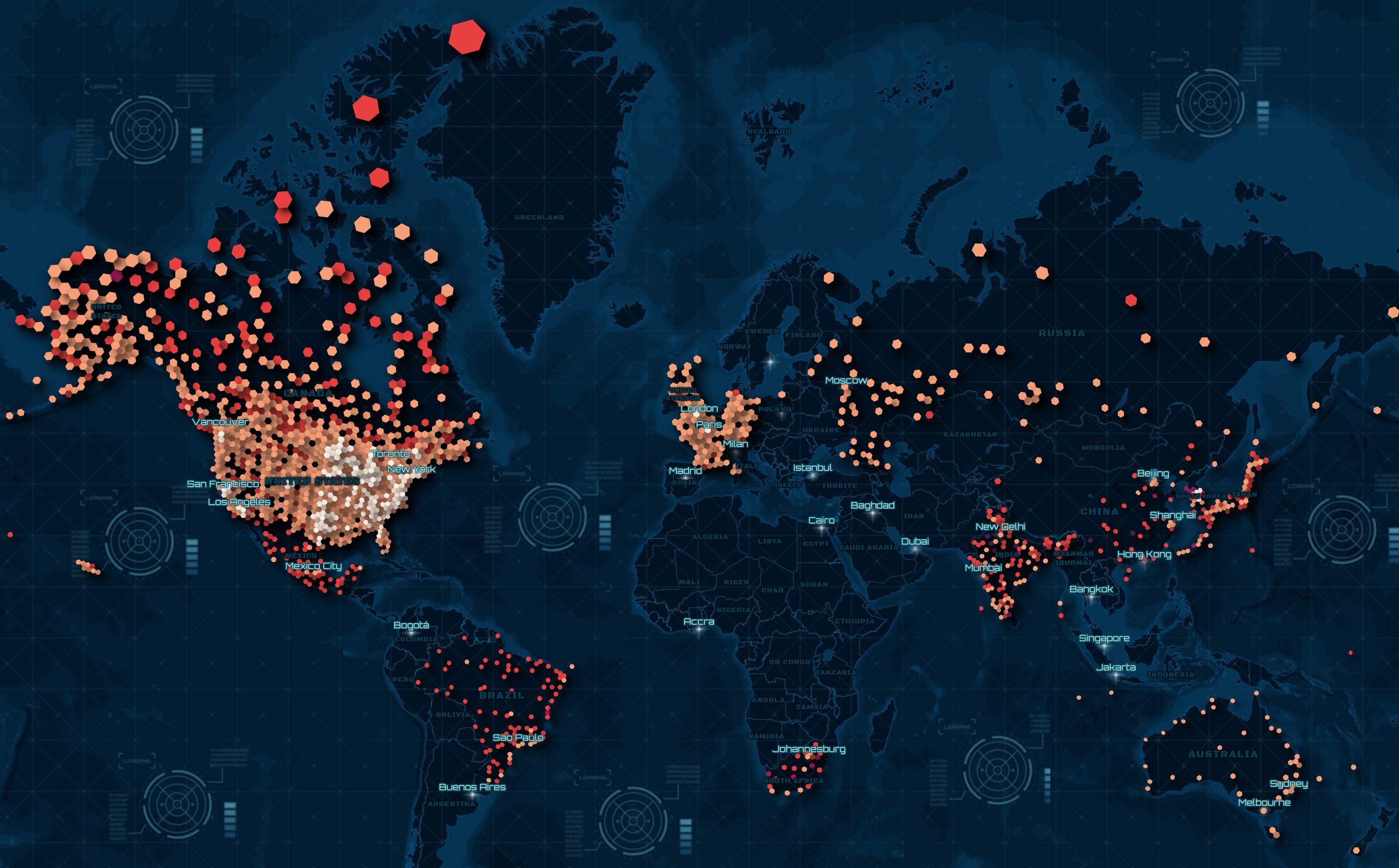
Below is a heatmap of their locations with the brightest hexagons representing the greatest number of observations.
CREATE OR REPLACE TABLE h3_stats AS
    SELECT   hexagon: H3_LATLNG_TO_CELL(
                        location.latitude,
                        location.longitude,
                        3),
             num_recs: COUNT(*)
    FROM     weather
    GROUP BY 1;

COPY (
    SELECT geometry: ST_ASWKB(H3_CELL_TO_BOUNDARY_WKT(hexagon)::geometry),
           num_recs
    FROM   h3_stats
) TO 'asos.h3s.parquet' (
        FORMAT 'PARQUET',
        CODEC  'ZSTD',
        COMPRESSION_LEVEL 22,
        ROW_GROUP_SIZE 15000);
Observations by Decade
I'll get the number of records per year in this dataset.
$ ~/duckdb asos.duckdb
CREATE OR REPLACE TABLE yearly_counts (
    year    INT,
    num_obs BIGINT
);
$ for YEAR in {1940..2026}; do
    echo $YEAR
    echo "INSERT INTO yearly_counts (year, num_obs)
          SELECT $YEAR,
                 COUNT(*)
          FROM 'https://data.source.coop/dynamical/asos-parquet/year=$YEAR/data.parquet'" \
        | ~/duckdb asos.duckdb
  done
There have been more than 1.75B observations across this entire dataset.
$ ~/duckdb asos.duckdb
SELECT SUM(num_obs)
FROM   yearly_counts;
┌────────────────┐
│  sum(num_obs)  │
│     int128     │
├────────────────┤
│   1750088324   │
│ (1.75 billion) │
└────────────────┘
Below are the largest number of observations seen within any one year within any given decade.
SELECT   decade: FLOOR(year / 10)::INT * 10,
         MAX(num_obs)
FROM     yearly_counts
GROUP BY 1
ORDER BY 1;
┌────────┬──────────────┐
│ decade │ max(num_obs) │
│ int32  │    int64     │
├────────┼──────────────┤
│   1940 │      5284124 │
│   1950 │      6046249 │
│   1960 │      5789299 │
│   1970 │     10288125 │
│   1980 │     12507342 │
│   1990 │     24676905 │
│   2000 │     49115404 │
│   2010 │     58220234 │
│   2020 │     59742202 │
└────────┴──────────────┘
I checked the latest forecast in this year's dataset as it was valid up to about 30 minutes before I ran this command.
$ ~/duckdb asos.duckdb
SELECT MAX(valid)
FROM   'https://data.source.coop/dynamical/asos-parquet/year=2026/data.parquet'
┌──────────────────────────┐
│       max("valid")       │
│ timestamp with time zone │
├──────────────────────────┤
│ 2026-05-26 20:40:00+03   │
└──────────────────────────┘