In May, the US Geological Survey (USGS) published version 8.1 of the U.S. Wind Turbine Database (USWTDB). The first version was published back in 2018 and it documents the location 76K+ wind turbines, their capabilities and associated project data across the US and its territories.
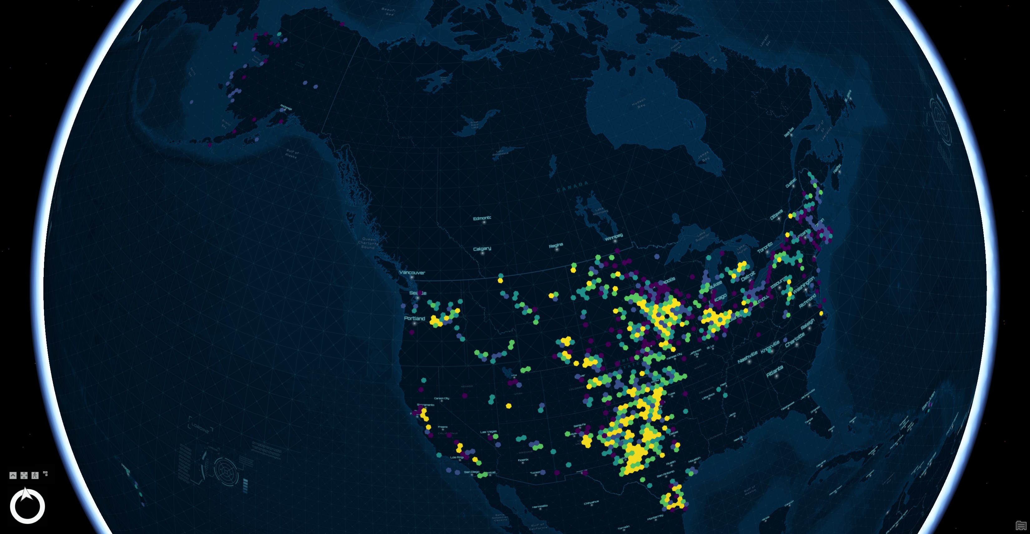
Below is a heatmap of their locations.
In this post, I'll walk through converting this dataset into Parquet and examining some of its features.
My Workstation
I'm using a 5.7 GHz AMD Ryzen 9 9950X CPU. It has 16 cores and 32 threads and 1.2 MB of L1, 16 MB of L2 and 64 MB of L3 cache. It has a liquid cooler attached and is housed in a spacious, full-sized Cooler Master HAF 700 computer case.
The system has 96 GB of DDR5 RAM clocked at 4,800 MT/s and a 5th-generation, Crucial T700 4 TB NVMe M.2 SSD which can read at speeds up to 12,400 MB/s. There is a heatsink on the SSD to help keep its temperature down. This is my system's C drive.
The system is powered by a 1,200-watt, fully modular Corsair Power Supply and is sat on an ASRock X870E Nova 90 Motherboard.
I'm running Ubuntu 24 LTS via Microsoft's Ubuntu for Windows on Windows 11 Pro. In case you're wondering why I don't run a Linux-based desktop as my primary work environment, I'm still using an Nvidia GTX 1080 GPU which has better driver support on Windows and ArcGIS Pro only supports Windows natively.
Installing Prerequisites
I'll use GDAL 3.9.3 and a few other tools to help analyse the data in this post.
$ sudo add-apt-repository ppa:ubuntugis/ubuntugis-unstable
$ sudo apt update
$ sudo apt install \
    gdal-bin \
    jq
I'll use DuckDB, along with its H3, JSON, Lindel, Parquet and Spatial extensions in this post.
$ cd ~
$ wget -c https://github.com/duckdb/duckdb/releases/download/v1.4.1/duckdb_cli-linux-amd64.zip
$ unzip -j duckdb_cli-linux-amd64.zip
$ chmod +x duckdb
$ ~/duckdb
INSTALL h3 FROM community;
INSTALL lindel FROM community;
INSTALL json;
INSTALL parquet;
INSTALL spatial;
I'll set up DuckDB to load every installed extension each time it launches.
$ vi ~/.duckdbrc
.timer on
.width 180
LOAD h3;
LOAD lindel;
LOAD json;
LOAD parquet;
LOAD spatial;
Most of the maps in this post were rendered with QGIS version 3.44. QGIS is a desktop application that runs on Windows, macOS and Linux. The application has grown in popularity in recent years and has ~15M application launches from users all around the world each month.
I used QGIS' Tile+ plugin to add basemaps from NASA's Blue Marble and Bing for spatial context.
I also used the following GeoJSON files for counties and states.
Downloading the Dataset
I'll download the dataset and convert it into Parquet.
The original field names contained a lot of acronyms and truncated names. I've renamed and restructured these for easier human consumption. I've taken all the values representing missing values and converted them into NULLs. I've also converted any magic numbers into English strings.
$ mkdir -p ~/usgs_wind
$ cd ~/usgs_wind

$ wget https://energy.usgs.gov/uswtdb/assets/data/uswtdbSHP.zip
$ unzip uswtdbSHP.zip
$ ~/duckdb
COPY (
    SELECT
        case_id: case_id::INT,
        eia_id:  IF(eia_id::TEXT='-9999', NULL, eia_id::INT),
        faa: {
            asn: IF(faa_asn='missing', NULL, faa_asn),
            ors: IF(faa_ors='missing', NULL, faa_ors),
        },
        project: {
            avg_turbine_capacity: IF(p_cap::TEXT='-9999.0', NULL, p_cap::DOUBLE),
            name:                 p_name,
            num_turbines:         p_tnum::INT,
            online_year:          IF(p_year::TEXT='-9999', NULL, p_year::INT),
        },
        geometry: geom,
        bbox:     {'xmin': ST_XMIN(ST_EXTENT(geom)),
                   'ymin': ST_YMIN(ST_EXTENT(geom)),
                   'xmax': ST_XMAX(ST_EXTENT(geom)),
                   'ymax': ST_YMAX(ST_EXTENT(geom))},
        location: {
            country: t_county,
            fips:    IF(t_fips::VARCHAR='NA', NULL, t_fips::VARCHAR),
            state:   t_state,
        },
        turbine: {
            capacity:          IF(t_cap::TEXT='-9999', NULL, t_cap::DOUBLE),
            attribute_confidence:
                CASE WHEN t_conf_atr = 1 THEN 'Low'
                     WHEN t_conf_atr = 2 THEN 'Medium'
                     WHEN t_conf_atr = 3 THEN 'High'
                END,
            location_confidence:
                CASE WHEN t_conf_loc = 1 THEN 'Low'
                     WHEN t_conf_loc = 2 THEN 'Medium'
                     WHEN t_conf_loc = 3 THEN 'High'
                END,
            hub_height:        IF(t_hh::TEXT='-9999.0', NULL, t_hh::DOUBLE),
            imagery: {
                captured_at:   t_img_date,
                provider:      t_img_src,
            },
            manufacturer:      IF(t_manu='missing', NULL, t_manu),
            model:             IF(t_model='missing', NULL, t_model),
            is_offshore:       t_offshore=1,
            rated_capacity: IF(t_rd::TEXT='-9999.0', NULL, t_rd::DOUBLE),
            retrofitted_year:  IF(t_retro_yr::TEXT='-9999', NULL, t_retro_yr::INT),
            is_retrofitted:    t_retrofit=1,
            rsa:               IF(t_rsa::TEXT='-9999.0', NULL, t_rsa::DOUBLE),
            ttlh:              IF(t_ttlh::TEXT='-9999.0', NULL, t_ttlh::DOUBLE),
        },
        usgs_pr_id:            IF(usgs_pr_id::TEXT='-9999', NULL, usgs_pr_id::INT),
    FROM ST_READ('uswtdb_V8_1_20250522.shx')
    ORDER BY HILBERT_ENCODE([ST_Y(ST_CENTROID(geom)),
                             ST_X(ST_CENTROID(geom))]::double[2])
) TO 'uswtdb_V8_1_20250522.parquet' (
        FORMAT 'PARQUET',
        CODEC  'ZSTD',
        COMPRESSION_LEVEL 22,
        ROW_GROUP_SIZE 15000);
Data Fluency
The following is an example record from this dataset.
$ echo "SELECT * EXCLUDE(bbox, faa, project, location, turbine),
               bbox::JSON     AS bbox,
               faa::JSON      AS faa,
               project::JSON  AS project,
               location::JSON AS location,
               turbine::JSON  AS turbine
        FROM   'uswtdb_V8_1_20250522.parquet'
        LIMIT  1" \
    | ~/duckdb -json \
    | jq -S .
[
  {
    "bbox": {
      "xmax": 144.72265600000003,
      "xmin": 144.72265600000003,
      "ymax": 13.389381000000071,
      "ymin": 13.389381000000071
    },
    "case_id": 3063607,
    "eia_id": null,
    "faa": {
      "asn": "2013-WTW-2712-OE",
      "ors": null
    },
    "geometry": "POINT (144.72265600000003 13.389381000000071)",
    "location": {
      "country": "Guam",
      "fips": "66010",
      "state": "GU"
    },
    "project": {
      "avg_turbine_capacity": 0.275,
      "name": "Guam Power Authority Wind Turbine",
      "num_turbines": 1,
      "online_year": 2016
    },
    "turbine": {
      "attribute_confidence": "High",
      "capacity": 275.0,
      "hub_height": 55.0,
      "imagery": {
        "captured_at": "2017-08-10",
        "provider": "Maxar"
      },
      "is_offshore": false,
      "is_retrofitted": false,
      "location_confidence": "High",
      "manufacturer": "Vergnet",
      "model": "GEV MP-C",
      "rated_capacity": 32.0,
      "retrofitted_year": null,
      "rsa": 804.25,
      "ttlh": 71.0
    },
    "usgs_pr_id": null
  }
]
Below are the field names, data types, percentages of NULLs per column, number of unique values and minimum and maximum values for each column.
$ ~/duckdb
SELECT   column_name,
         column_type,
         null_percentage,
         approx_unique,
         min,
         max
FROM     (SUMMARIZE
          SELECT case_id,
                 eia_id,
                 faa.*,
                 location.*,
                 project.*,
                 turbine.* EXCLUDE(imagery),
                 turbine.imagery.captured_at,
                 turbine.imagery.provider,
                 usgs_pr_id,
          FROM   'uswtdb_V8_1_20250522.parquet')
ORDER BY 1;
┌──────────────────────┬─────────────┬─────────────────┬───────────────┬──────────────────┬─────────────────────┐
│     column_name      │ column_type │ null_percentage │ approx_unique │       min        │         max         │
│       varchar        │   varchar   │  decimal(9,2)   │     int64     │     varchar      │       varchar       │
├──────────────────────┼─────────────┼─────────────────┼───────────────┼──────────────────┼─────────────────────┤
│ asn                  │ VARCHAR     │            5.37 │         50703 │ 1987-AGL-900-OE  │ 2025-WTW-669-OE     │
│ attribute_confidence │ VARCHAR     │            0.00 │             3 │ High             │ Medium              │
│ avg_turbine_capacity │ DOUBLE      │            3.86 │           762 │ 0.05             │ 1055.6              │
│ capacity             │ DOUBLE      │            5.25 │           111 │ 50.0             │ 13000.0             │
│ captured_at          │ DATE        │            0.00 │          1669 │ 1970-01-01       │ 2025-03-25          │
│ case_id              │ INTEGER     │            0.00 │         78762 │ 3000001          │ 3140627             │
│ country              │ VARCHAR     │            0.00 │           566 │ Adair County     │ Zapata County       │
│ eia_id               │ INTEGER     │            5.17 │          1359 │ 90               │ 68318               │
│ fips                 │ VARCHAR     │            0.08 │           637 │ 02013            │ 72133               │
│ hub_height           │ DOUBLE      │            5.99 │           111 │ 19.0             │ 136.0               │
│ is_offshore          │ BOOLEAN     │            0.00 │             2 │ false            │ true                │
│ is_retrofitted       │ BOOLEAN     │            0.00 │             2 │ false            │ true                │
│ location_confidence  │ VARCHAR     │            0.00 │             3 │ High             │ Medium              │
│ manufacturer         │ VARCHAR     │            5.48 │            60 │ AAER             │ Zond                │
│ model                │ VARCHAR     │            5.65 │           318 │ 1.5-70.5         │ Zond                │
│ name                 │ VARCHAR     │            0.00 │          1806 │ 25 Mile Creek    │ unknown Yuma County │
│ num_turbines         │ INTEGER     │            0.00 │           192 │ 1                │ 713                 │
│ online_year          │ INTEGER     │            1.20 │            42 │ 1982             │ 2025                │
│ ors                  │ VARCHAR     │            5.91 │         72659 │ 02-000669        │ 56-064307           │
│ provider             │ VARCHAR     │            0.00 │             5 │ Bing Maps Aerial │ Planet              │
│ rated_capacity       │ DOUBLE      │            5.88 │           113 │ 13.4             │ 200.0               │
│ retrofitted_year     │ INTEGER     │           89.39 │             9 │ 2015             │ 2023                │
│ rsa                  │ DOUBLE      │            5.88 │           121 │ 141.03           │ 31415.93            │
│ state                │ VARCHAR     │            0.00 │            55 │ AK               │ WY                  │
│ ttlh                 │ DOUBLE      │            5.99 │           235 │ 31.0             │ 210.9               │
│ usgs_pr_id           │ INTEGER     │           51.44 │         36701 │ 1                │ 49135               │
├──────────────────────┴─────────────┴─────────────────┴───────────────┴──────────────────┴─────────────────────┤
│ 26 rows                                                                                             6 columns │
└───────────────────────────────────────────────────────────────────────────────────────────────────────────────┘
Turbines
Below I'll generate a heatmap of turbine installation locations.
$ ~/duckdb
CREATE OR REPLACE TABLE h3_4_stats AS
    SELECT   h3_4: H3_LATLNG_TO_CELL(
                        bbox.ymin,
                        bbox.xmin,
                        4),
             COUNT(*) num_turbines
    FROM     'uswtdb_V8_1_20250522.parquet'
    GROUP BY 1;

COPY (
    SELECT ST_ASWKB(H3_CELL_TO_BOUNDARY_WKT(h3_4)::geometry) geometry,
           num_turbines
    FROM   h3_4_stats
    WHERE  ST_XMIN(geometry::geometry) BETWEEN -179 AND 179
    AND    ST_XMAX(geometry::geometry) BETWEEN -179 AND 179
) TO 'turbines.h3_4.gpkg'
  WITH (FORMAT GDAL,
        DRIVER 'GPKG',
        LAYER_CREATION_OPTIONS 'WRITE_BBOX=YES');
The following was needed for ArcGIS Pro to recognise the projection of the above hexagons properly.
$ ogr2ogr \
    -f GPKG \
    -a_srs EPSG:4326 \
    turbines.h3_4.4326.gpkg \
    turbines.h3_4.gpkg
There are 63 unique manufactures listed in this dataset. These are the ones with the most and least number of turbines installed.
$ ~/duckdb
SELECT   num_turbines: COUNT(*),
         turbine.manufacturer
FROM     'uswtdb_V8_1_20250522.parquet'
GROUP BY 2
ORDER BY 1 DESC;
┌──────────────┬──────────────────────────────────────────────────────────────────────────┐
│ num_turbines │                               manufacturer                               │
│    int64     │                                 varchar                                  │
├──────────────┼──────────────────────────────────────────────────────────────────────────┤
│        34613 │ GE Wind                                                                  │
│        17649 │ Vestas                                                                   │
│         4689 │ Siemens                                                                  │
│         4167 │ NULL                                                                     │
│         2999 │ Gamesa                                                                   │
│         2765 │ Siemens Gamesa Renewable Energy                                          │
│         2214 │ Mitsubishi                                                               │
│         1917 │ Nordex                                                                   │
│         1190 │ Suzlon                                                                   │
│          758 │ Acciona                                                                  │
│            · │    ·                                                                     │
│            · │    ·                                                                     │
│            · │    ·                                                                     │
│            1 │ Wind Energy Solutions                                                    │
│            1 │ Bergey Energy                                                            │
│            1 │ Leitner Poma                                                             │
│            1 │ Norwin                                                                   │
│            1 │ DWT                                                                      │
│            1 │ Unison                                                                   │
│            1 │ Silver Eagle                                                             │
│            1 │ Changzhou Railcar Propulsion Engineering Research and Development Center │
│            1 │ Wincon                                                                   │
│            1 │ Renewtech LLC                                                            │
├──────────────┴──────────────────────────────────────────────────────────────────────────┤
│ 64 rows (20 shown)                                                            2 columns │
└─────────────────────────────────────────────────────────────────────────────────────────┘
Below are the number of turbines by manufacturer where at least 40 were installed in any one decade.
.maxrows 40

WITH a AS (
    SELECT   num_turbines: COUNT(*),
             decade:       (project.online_year / 10)::INT * 10,
             manufacturer: turbine.manufacturer
    FROM     'uswtdb_V8_1_20250522.parquet'
    WHERE    turbine.manufacturer IS NOT NULL
    GROUP BY 2, 3
    HAVING   num_turbines > 40
    ORDER BY 1 DESC
)
PIVOT    a
ON       decade
USING    SUM(num_turbines)
GROUP BY manufacturer
ORDER BY manufacturer;
┌─────────────────────────────────┬────────┬────────┬────────┬────────┬────────┐
│          manufacturer           │  1980  │  1990  │  2000  │  2010  │  2020  │
│             varchar             │ int128 │ int128 │ int128 │ int128 │ int128 │
├─────────────────────────────────┼────────┼────────┼────────┼────────┼────────┤
│ Acciona                         │   NULL │   NULL │   NULL │    603 │    155 │
│ Bonus                           │    152 │     55 │     97 │   NULL │   NULL │
│ Clipper                         │   NULL │   NULL │   NULL │    198 │   NULL │
│ Enron                           │   NULL │   NULL │    395 │   NULL │   NULL │
│ GE Wind                         │   NULL │   NULL │   1397 │  15234 │  17950 │
│ Gamesa                          │   NULL │   NULL │    386 │   1842 │    771 │
│ Goldwind                        │   NULL │   NULL │   NULL │    106 │     88 │
│ Goldwind Americas               │   NULL │   NULL │   NULL │   NULL │     48 │
│ Micon                           │   NULL │    198 │   NULL │   NULL │   NULL │
│ Mitsubishi                      │   NULL │   NULL │    396 │   1818 │   NULL │
│ NEG Micon                       │   NULL │   NULL │    440 │   NULL │   NULL │
│ Nordex                          │   NULL │   NULL │     41 │    265 │   1611 │
│ Nordtank                        │    207 │   NULL │   NULL │   NULL │   NULL │
│ Northern Power Systems          │   NULL │   NULL │   NULL │     92 │   NULL │
│ REpower                         │   NULL │   NULL │   NULL │    559 │   NULL │
│ Siemens                         │   NULL │   NULL │   NULL │   3300 │   1389 │
│ Siemens Gamesa Renewable Energy │   NULL │   NULL │    314 │    450 │   2001 │
│ Suzlon                          │   NULL │   NULL │   NULL │   1172 │   NULL │
│ Vestas                          │     48 │   NULL │   1532 │   4787 │  11265 │
│ Zond                            │   NULL │   NULL │     83 │   NULL │   NULL │
├─────────────────────────────────┴────────┴────────┴────────┴────────┴────────┤
│ 20 rows                                                            6 columns │
└──────────────────────────────────────────────────────────────────────────────┘
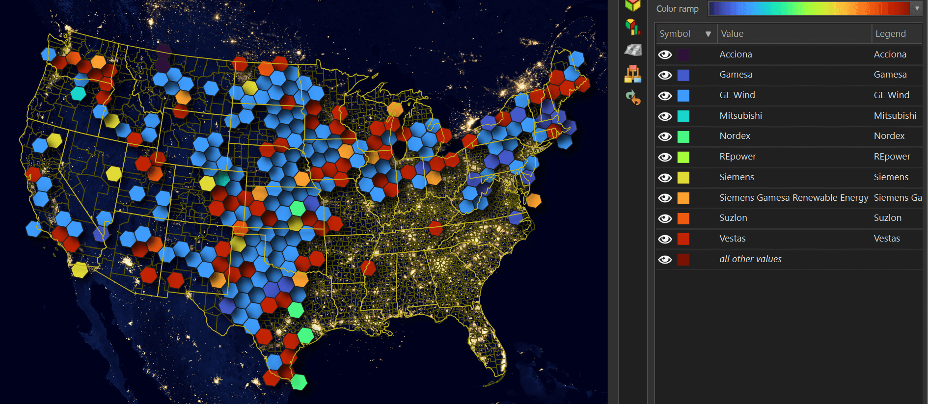
Below I'll plot out the top manufacturer per hexagon in the lower 48 states among the overall top ten.
CREATE OR REPLACE TABLE top_manufacturers AS
    SELECT   num_turbines: COUNT(*),
             manufacturer: turbine.manufacturer
    FROM     'uswtdb_V8_1_20250522.parquet'
    WHERE    turbine.manufacturer IS NOT NULL
    GROUP BY 2
    ORDER BY 1 DESC
    LIMIT    10;

CREATE OR REPLACE TABLE h3_3s AS
    WITH b AS (
        WITH a AS (
            SELECT   H3_LATLNG_TO_CELL(bbox.ymin,
                                       bbox.xmin,
                                       3) h3_3,
                     manufacturer: turbine.manufacturer,
                     COUNT(*) num_recs
            FROM     'uswtdb_V8_1_20250522.parquet'
            WHERE    turbine.manufacturer IN (
                SELECT DISTINCT manufacturer
                FROM   top_manufacturers
            )
            GROUP BY 1, 2
        )
        SELECT *,
               ROW_NUMBER() OVER (PARTITION BY h3_3
                                  ORDER BY     num_recs DESC) AS rn
        FROM   a
    )
    FROM     b
    WHERE    rn = 1
    ORDER BY num_recs DESC;

COPY (
    SELECT geom: H3_CELL_TO_BOUNDARY_WKT(h3_3)::GEOMETRY,
           manufacturer
    FROM   h3_3s
    WHERE  ST_XMIN(geom::GEOMETRY) BETWEEN -179 AND 179
    AND    ST_XMAX(geom::GEOMETRY) BETWEEN -179 AND 179
) TO 'turbine.top_manufacturer.h3_3.parquet' (
    FORMAT 'PARQUET',
    CODEC  'ZSTD',
    COMPRESSION_LEVEL 22,
    ROW_GROUP_SIZE 15000);
Only 67 turbines in this dataset are listed as being offshore.
SELECT   COUNT(*),
         turbine.is_offshore
FROM     'uswtdb_V8_1_20250522.parquet'
GROUP BY 2;
┌──────────────┬─────────────┐
│ count_star() │ is_offshore │
│    int64     │   boolean   │
├──────────────┼─────────────┤
│        75984 │ false       │
│           67 │ true        │
└──────────────┴─────────────┘
Below are the top 20 states by their total GW of installed capacity, number of turbines and distinct manufacturers represented.
SELECT   location.state,
         gw:                ROUND(SUM(turbine.capacity) / 1000 ** 2, 2),
         num_turbines:      COUNT(*),
         num_manufacturers: COUNT(DISTINCT turbine.manufacturer)
FROM     'uswtdb_V8_1_20250522.parquet'
GROUP BY 1
ORDER BY 2 DESC
LIMIT    20;
┌─────────┬────────┬──────────────┬───────────────────┐
│  state  │   gw   │ num_turbines │ num_manufacturers │
│ varchar │ double │    int64     │       int64       │
├─────────┼────────┼──────────────┼───────────────────┤
│ TX      │  42.77 │        19415 │                22 │
│ IA      │  13.18 │         6472 │                22 │
│ OK      │  12.72 │         5597 │                13 │
│ KS      │    9.1 │         4415 │                11 │
│ IL      │   7.92 │         3837 │                16 │
│ CA      │   6.05 │         5510 │                18 │
│ CO      │   5.39 │         2908 │                12 │
│ MN      │   4.83 │         2736 │                19 │
│ ND      │   4.48 │         2169 │                 9 │
│ NM      │   4.33 │         2305 │                 7 │
│ OR      │    4.1 │         2173 │                 9 │
│ MI      │   3.73 │         1715 │                 9 │
│ WY      │   3.65 │         1713 │                 6 │
│ IN      │   3.62 │         1651 │                12 │
│ SD      │   3.62 │         1503 │                 9 │
│ NE      │   3.42 │         1504 │                 6 │
│ WA      │    3.4 │         1825 │                 9 │
│ NY      │   2.74 │         1429 │                13 │
│ MO      │   2.44 │         1108 │                 5 │
│ MT      │   1.89 │         1039 │                 7 │
├─────────┴────────┴──────────────┴───────────────────┤
│ 20 rows                                   4 columns │
└─────────────────────────────────────────────────────┘
Below is the ever-increasing capacity of turbines in MW over the decades.
WITH a AS (
    SELECT   decade:       (project.online_year / 10)::INT * 10,
             mw:           CEIL(turbine.capacity / 1000)::INT,
             num_turbines: COUNT(*)
    FROM     'uswtdb_V8_1_20250522.parquet'
    WHERE    turbine.capacity IS NOT NULL
    GROUP BY 1, 2
)
PIVOT    a
ON       decade
USING    SUM(num_turbines)
GROUP BY mw
ORDER BY mw;
┌───────┬────────┬────────┬────────┬────────┬────────┐
│  mw   │  1980  │  1990  │  2000  │  2010  │  2020  │
│ int32 │ int128 │ int128 │ int128 │ int128 │ int128 │
├───────┼────────┼────────┼────────┼────────┼────────┤
│     1 │    419 │    434 │   2750 │   1514 │     45 │
│     2 │   NULL │   NULL │   2359 │  20972 │  10223 │
│     3 │   NULL │   NULL │      1 │   7969 │  18733 │
│     4 │   NULL │   NULL │   NULL │    207 │   3588 │
│     5 │   NULL │   NULL │     38 │     19 │   2514 │
│     6 │   NULL │   NULL │   NULL │   NULL │    215 │
│    11 │   NULL │   NULL │   NULL │   NULL │     12 │
│    13 │   NULL │   NULL │   NULL │   NULL │      9 │
└───────┴────────┴────────┴────────┴────────┴────────┘
Of the 76K turbines in this dataset, 67K have a high confidence rating for both their location and attributes.
WITH a AS (
    SELECT   attribute:    turbine.attribute_confidence,
             location:     turbine.location_confidence,
             num_turbines: COUNT(*)
    FROM     'uswtdb_V8_1_20250522.parquet'
    GROUP BY 1, 2
    ORDER BY 3 DESC
)
PIVOT    a
ON       attribute,
USING    SUM(num_turbines)
GROUP BY location
ORDER BY location;
┌──────────┬────────┬────────┬────────┐
│ location │  High  │  Low   │ Medium │
│ varchar  │ int128 │ int128 │ int128 │
├──────────┼────────┼────────┼────────┤
│ High     │  67060 │   2924 │   4472 │
│ Low      │    137 │   1256 │    141 │
│ Medium   │      1 │     60 │   NULL │
└──────────┴────────┴────────┴────────┘
Project Footprints
Each turbine record contains denormalised project information. Below I'll generate the footprints for each project.
I'll group the projects by level-3 hexagons and name to generate their geographical footprints. This helps avoid country-wide overlaps that would result from grouping by name alone.
$ ~/duckdb
COPY (
    SELECT   h3_3: H3_LATLNG_TO_CELL(bbox.ymin,
                                     bbox.xmin,
                                     3),
             project_name: project.name,
             geometry: {
                'min_x': MIN(ST_X(geometry)),
                'min_y': MIN(ST_Y(geometry)),
                'max_x': MAX(ST_X(geometry)),
                'max_y': MAX(ST_Y(geometry))}::BOX_2D::GEOMETRY
    FROM     READ_PARQUET('uswtdb_V8_1_20250522.parquet')
    GROUP BY 1, 2
) TO 'projects.parquet' (
        FORMAT 'PARQUET',
        CODEC  'ZSTD',
        COMPRESSION_LEVEL 22,
        ROW_GROUP_SIZE 15000);
A total of 2,008 distinct projects were returned. Below are a few of these projects in Texas.
