A year after the invention of the Laser in 1960, the first laser imaging, detection, and ranging (LiDAR) system was attached to an aircraft by the Hughes Aircraft Company, a major aerospace and defense contractor at the time. Since then, LiDAR has gone on to be used to scan everything surrounding self-driving cars, entire countries and even objects in space.
LiDAR is unique in that it not only measures RGB values of the surfaces it scans but it can also identify the material hit as well. It knows if it hits the ground, a building, vegetation or a body of water. This makes its resulting Point Cloud datasets very rich in a way that camera photos alone couldn't match.
Once expensive LiDAR scanners are now becoming more affordable to individuals and small businesses. Apple includes a LiDAR camera in the iPhone 12, 13 and 14 Pro and Pro Max models as well as the iPad Pro. That said, they haven't made the raw LiDAR data available via an API yet. Samsung did have a LiDAR sensor in their Galaxy S20 phone but dropped it when the S21 was released two years ago. DJI sell the Zenmuse L2, a LiDAR + RGB camera for ~€14K. There are also software techniques that can produce Point Clouds from regular phone images.
There are three file formats that you'll find a lot in the LiDAR world. LiDAR scanners typically produce data in LAS file format. The LAZ file format is the compressed version of LAS. Cloud-optimised Point Cloud (COPC) files are LAZ files but with the point data organised in a clustered octree.
Getting a hold of free LiDAR data is surprisingly easy. The United States Geological Survey (USGS) has published 300 TB of LiDAR scans on AWS S3. Audi published 2 TB of LiDAR and regular camera imagery on AWS S3. This was from 12 cameras that were attached to an Audi Q7 e-tron that drove three separate trips in 2018 and 2019. I've also seen several self-driving-focused datasets being offered by Ford, Lyft, Motional and Waymo. Finally, the Estonian Land Board has published country-wide scans yearly going back to 2016.
In this post, I'll download and examine the Estonian Land Board's 2022 LiDAR scan of Tallinn's Old Town.
Installing Prerequisites
The following was run on Ubuntu for Windows which is based on Ubuntu 20.04 LTS. The system is powered by an Intel Core i5 4670K running at 3.40 GHz and has 32 GB of RAM. The primary partition is a 2 TB Samsung 870 QVO SSD.
I'll be using Python as well as Point Data Abstraction Library (PDAL) to help out with some transformations and analysis in this post. PDAL is made up of over 250K lines of C++ and has been in active development for the past 12 years.
$ sudo apt update
$ sudo apt install \
    jq \
    pdal \
    python3-pip \
    python3-virtualenv
$ virtualenv ~/.lidar
$ source ~/.lidar/bin/activate
$ python -m pip install \
    copclib
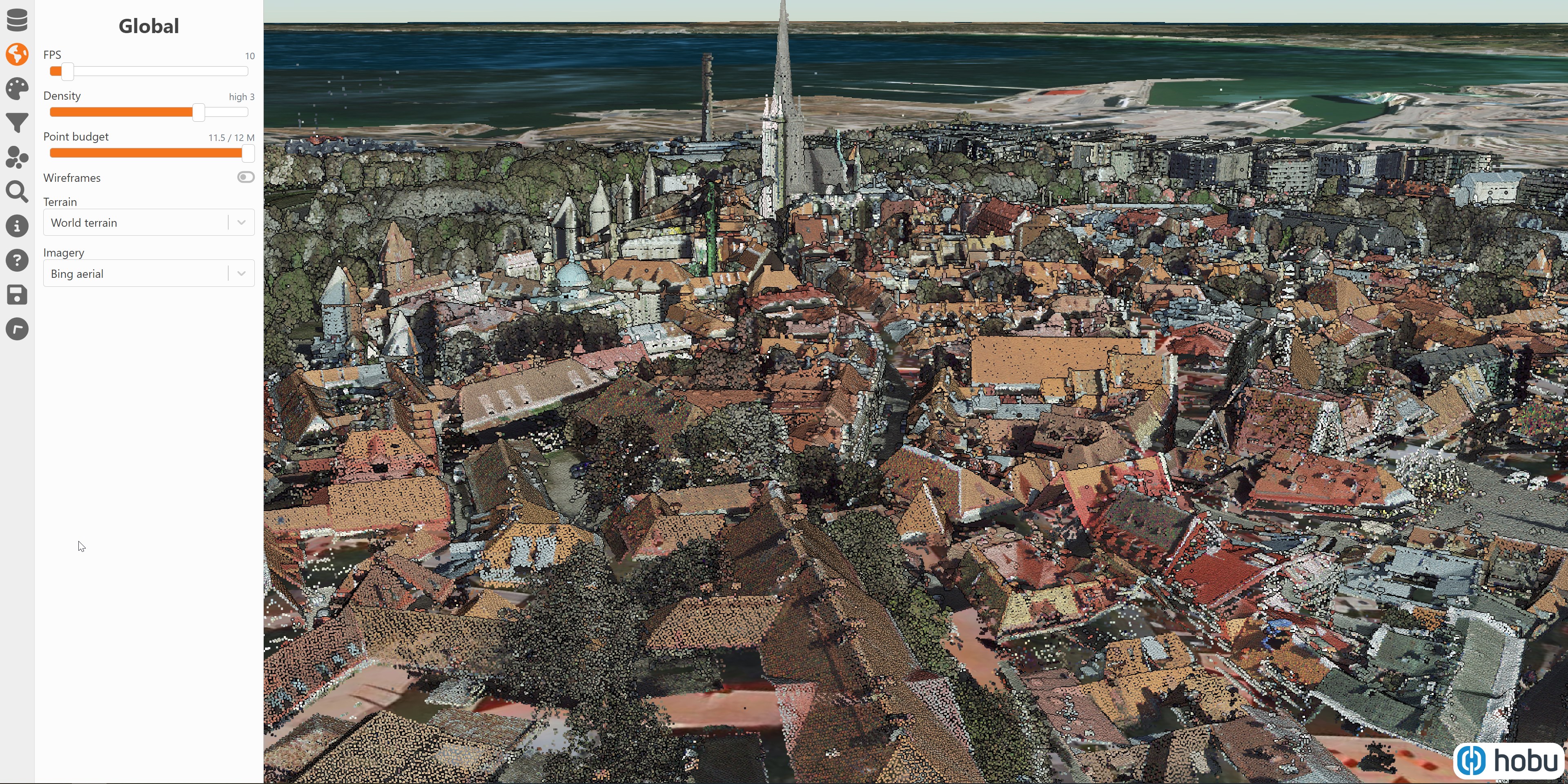
The maps in this post were rendered with QGIS version 3.34. QGIS is a desktop application that runs on Windows, macOS and Linux. I used QGIS' Tile+ plugin to add satellite basemaps.
The version of PDAL installed on Ubuntu for Windows is 2.0.1 which was released on Aug 23, 2019. QGIS 3.34 ships with PDAL 2.5.5 which was released in June.
Downloading Estonian LiDAR Data
Estonia has a card-page system to identify grid locations. I loaded the 1.3 MB Shapefile of this grid into QGIS and rendered it on top of Esri's World Imagery Basemap centred on Tallinn's Old Town.

Cell 589542 covers the area of interest in Tallinn's Old Town that I'm after. I submitted that card-page number to the Estonian Land Board's LiDAR asset search form and it came back with 18 LAZ files. These are the LAZ file sizes in MB broken down by year and collection type.
Year | madal | mets   | tava
-----|-------|--------|------
2008 |   4.8 |        |
2009 |       |        | 1.6
2012 |       |        | 1.6
2013 |       |        | 1.8
2014 |   8.5 |        |
2015 |       |        | 1.8
2016 |   4.2 |        | 613.4
2017 | 127.0 |        |
2018 | 168.0 |    8.2 |
2019 | 208.0 |        |
2020 | 247.9 |        | 28.2
2021 | 302.5 |        |
2022 | 290.3 |   10.4 |
2023 | 257.0 |        |
Estonian was the 4th language I studied and I rarely use it day-to-day so forgive the following attempt at translating the above. "mets" is Estonian for forest, "tava" can mean observation and "madal" probably means "base" in Estonian but it can also mean low, flat or shallow. I'm not sure what the Land Board was intending to describe but the "madal" file has the Point Clouds I'm after. For this exercise, I'll be using the 589542_2022_madal.laz file.
I'll use PDAL to convert the 290 MB LAZ file into a 187 MB Cloud-Optimised Point Clouds (COPC) file.
$ pdal translate \
    589542_2022_madal.laz \
    589542_2022_madal.copc.laz
With the COPC file generated, I can render it on https://viewer.copc.io. This website lets me fly around a 3D rendering of the LiDAR scan, turn points on and off based on classification and colour-code points based on a wide variety of attributes.
Examining the LiDAR Scan
Below are the projection settings for the file.
$ pdal info \
        --summary \
        589542_2022_madal.laz \
    | jq -S .summary.srs.prettywkt \
    | xargs -0 printf '%b\n'
"PROJCS["Estonian Coordinate System of 1997",
    GEOGCS["EST97",
        DATUM["Estonia_1997",
            SPHEROID["GRS 1980",6378137,298.257222101,
                AUTHORITY["EPSG","7019"]],
            AUTHORITY["EPSG","6180"]],
        PRIMEM["Greenwich",0,
            AUTHORITY["EPSG","8901"]],
        UNIT["degree",0.0174532925199433,
            AUTHORITY["EPSG","9122"]],
        AUTHORITY["EPSG","4180"]],
    PROJECTION["Lambert_Conformal_Conic_2SP"],
    PARAMETER["latitude_of_origin",57.5175539305556],
    PARAMETER["central_meridian",24],
    PARAMETER["standard_parallel_1",59.3333333333333],
    PARAMETER["standard_parallel_2",58],
    PARAMETER["false_easting",500000],
    PARAMETER["false_northing",6375000],
    UNIT["metre",1,
        AUTHORITY["EPSG","9001"]],
    AXIS["Northing",NORTH],
    AXIS["Easting",EAST],
    AUTHORITY["EPSG","3301"]]"
Below I'll extract the boundary information for the file.
$ pdal info \
        589542_2022_madal.laz \
        --boundary \
    | jq -S '.boundary|del(.boundary_json)'
{
  "area": 1010041.23,
  "avg_pt_per_sq_unit": 0.1064309265,
  "avg_pt_spacing": 0.1879944788,
  "boundary": "POLYGON ((542011.54 6588995.9,543001.14 6588995.9,543001.14 6590006.1,541999.59 6590002.0,541997.19 6589004.2,542011.54 6588995.9))",
  "density": 28.29500733,
  "edge_length": 0,
  "estimated_edge": 8.280414523,
  "hex_offsets": "MULTIPOINT (0 0, -2.39035 4.14021, 0 8.28041, 4.7807 8.28041, 7.17105 4.14021, 4.7807 0)",
  "sample_size": 5000,
  "threshold": 15
}
I'll extract the first point to show all the fields contained within this file.
$ pdal info \
        589542_2022_madal.laz \
        -p 0 \
    | jq -S '.points.point'
{
  "Amplitude": 15.61,
  "Blue": 14848,
  "ClassFlags": 0,
  "Classification": 6,
  "Deviation": 11,
  "EdgeOfFlightLine": 0,
  "GpsTime": 335088203.3,
  "Green": 18432,
  "Infrared": 25344,
  "Intensity": 51182,
  "NumberOfReturns": 1,
  "PointId": 0,
  "PointSourceId": 22292,
  "Pulse width": 0,
  "Red": 27136,
  "Reflectance": -1.56,
  "ReturnNumber": 1,
  "ScanAngleRank": 0.7680000067,
  "ScanChannel": 0,
  "ScanDirectionFlag": 0,
  "UserData": 122,
  "X": 542099.98,
  "Y": 6589000.02,
  "Z": 36.88
}
Below I'll count the number of points for each classification. I referred to the LAZ 1.4 Specification for the lookup values.
$ python3
from collections import Counter

import copclib as copc


reader = copc.FileReader('589542_2022_madal.copc.laz')
node   = reader.FindNode(copc.VoxelKey(0, 0, 0, 0))
points = reader.GetPoints(node)

asprs_point_classes = {
    0:  'Created, never classified',
    1:  'Unclassified',
    2:  'Ground',
    3:  'Low Vegetation',
    4:  'Medium Vegetation',
    5:  'High Vegetation',
    6:  'Building',
    7:  'Low Point (noise)',
    8:  'Model Key-point (mass point)',
    9:  'Water',
    10: 'Rail',
    11: 'Road Surface',
    12: 'Overlap Points',
    13: 'Wire - Guard (Shield)',
    14: 'Wire - Conductor (Phase)',
    15: 'Transmission Tower',
    16: 'Wire-structure Connector (e.g. Insulator)',
    17: 'Bridge Deck',
    18: 'High Noise',
    # 19 - 63: Reserved for ASPRS Definition
    # 64 - 255: User definable
}

def get_name(num):
    if num not in asprs_point_classes.keys():
        if num > 18 and num < 64:
            return 'Reserved for ASPRS Definition'
        elif num > 63 and num < 256:
            return 'User defined'

        return None
    else:
        return asprs_point_classes[num]


print(Counter(['%s (%d)' % (get_name(point.classification),
                            point.classification)
               for point in points]).most_common())
[('High Vegetation (5)', 46184),
 ('Ground (2)', 27052),
 ('Building (6)', 20909),
 ('Unclassified (1)', 13169),
 ('Low Point (noise) (7)', 509),
 ('High Noise (18)', 166),
 ('Water (9)', 2)]
There are between 20 - 46K points for buildings, the ground and vegetation but there are also 13K unclassified points.
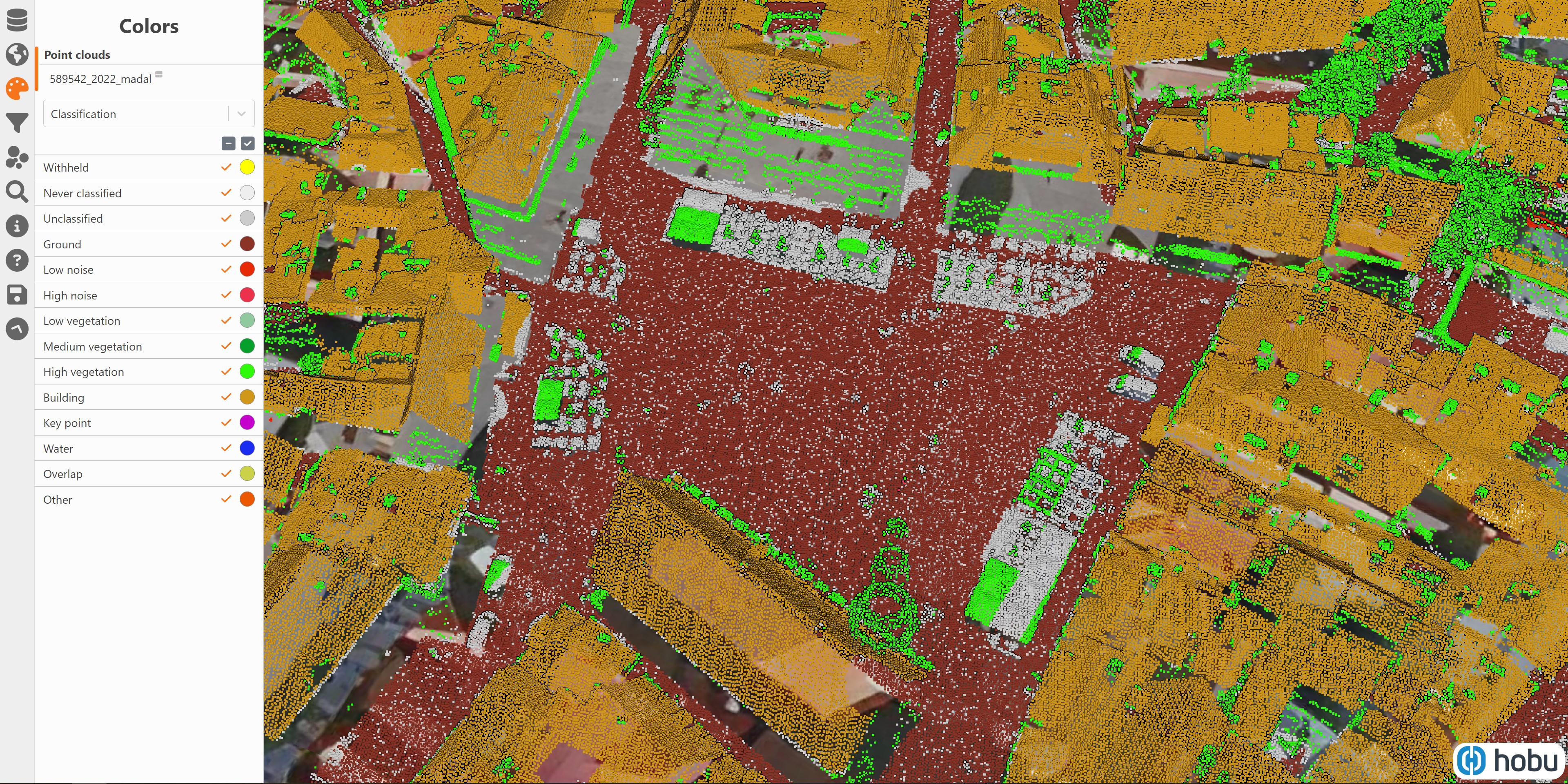
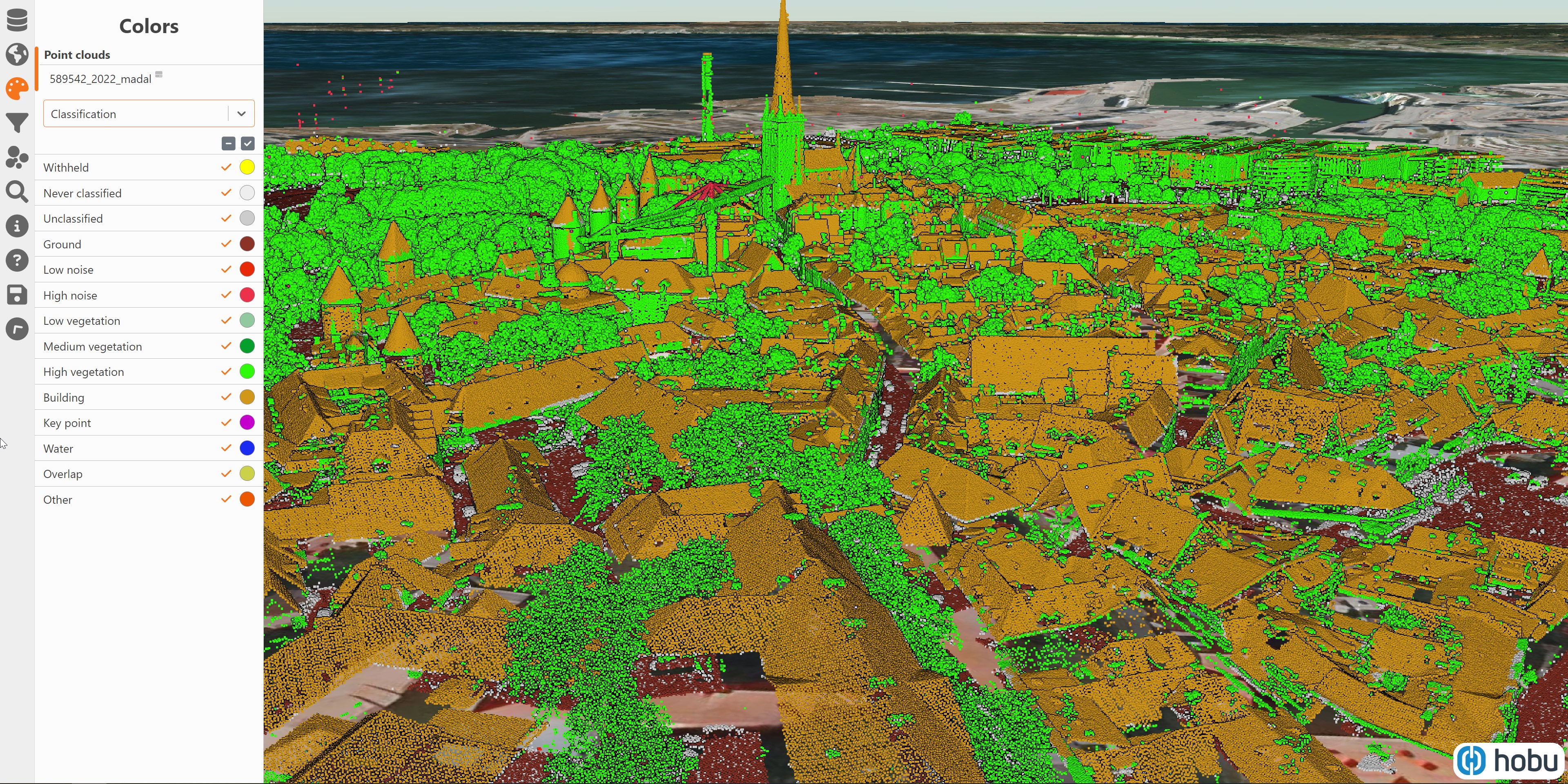
Below I've colour-coded the points by classification. The legend is to the left.
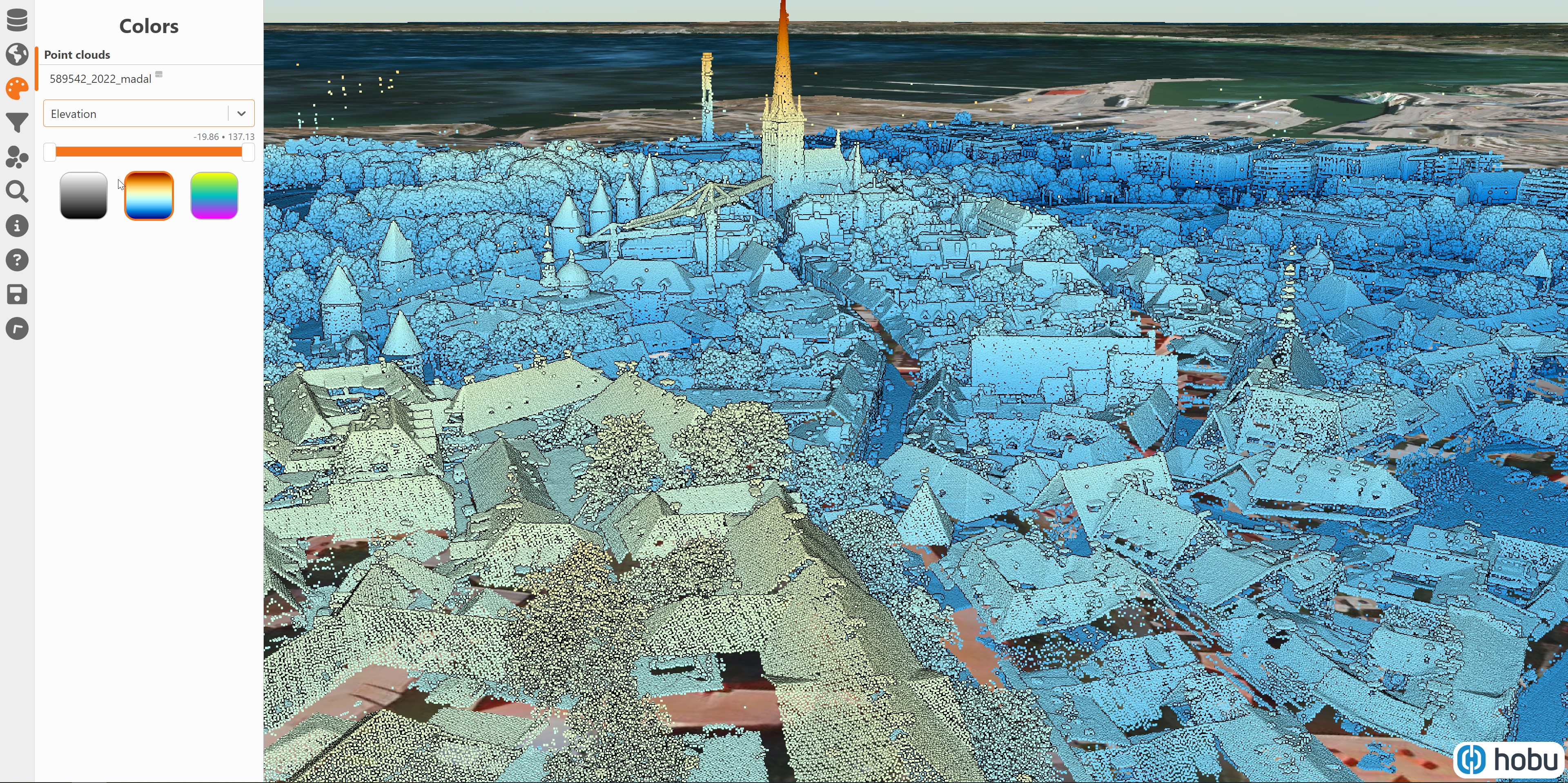
Below the points are colour-coded by elevation.
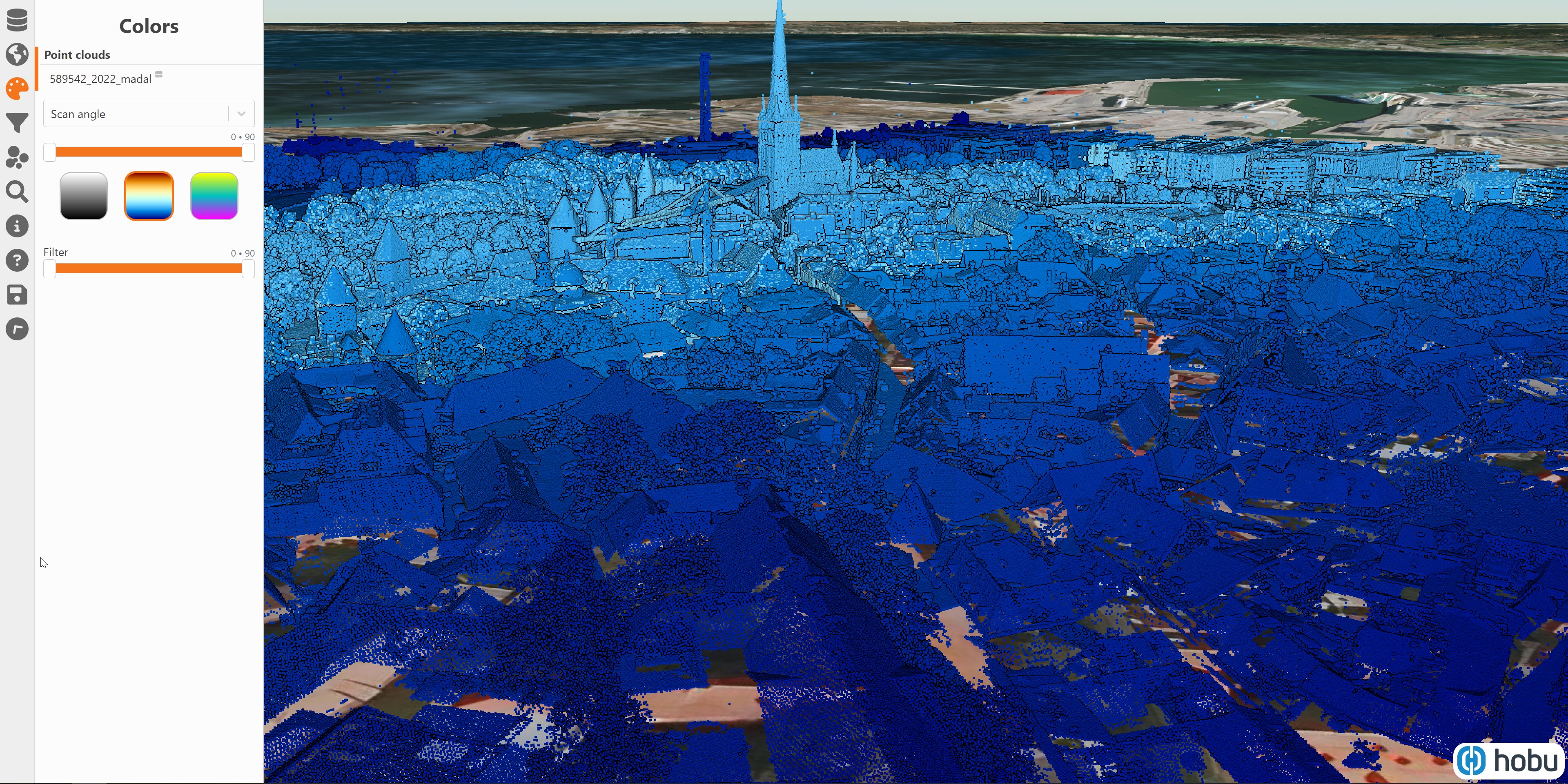
Below the points are colour-coded by the angle at which they were scanned.
Separating Everything in QGIS
Below is every point in the COPC file rendered together in QGIS.

I've duplicated that layer three times and applied filters to each layer. One layer will have only buildings, another will have only roads, a third will only have vegetation and the fourth will contain every else. QGIS has text labels in its filter dialog so you don't have to remember the number of each classification.

Below are the buildings rendered on their own layer separately from everything else.

Below is the ground being rendered on its own. Most of the outdoor seating appears here as well.

Below are the vegetation points. Notice how the red roofs of the buildings and their outer walls leak into these points. Some of the outdoor seating appears here as well.

Below is everything else. These are the 13K unclassified points. The bulk of the outdoor seating points can be seen here.

This is the RGB rendering of Tallinn's Town Hall Square where a lot of outdoor seating can be found.

This is the same area but with the points colour-coded by classification. Most of the wooden floors for the seating areas are unclassified. The canopies are classed as high vegetation as are the van windshields and parts of the outer walls of the buildings. The ground is mostly classed correctly but there is a layer of unclassified points covering it like snow flakes.